General Circulation Experiment at MIT
We are two graduate students from MIT and we would like to share our experiences in carrying out the General Circulation Experiment in our GFD laboratory here.
Introduction
It is a well-established observation that there is more solar incoming radiation at the equator than at the poles and that the radiative heat loss at the poles is much stronger than at the equator. In order to keep a steady state system, there needs to be meridional, i.e. poleward, heat transport in the earth system. Both the atmosphere and the ocean contribute to this, but the mechanisms are quite different depending on the Rossby radius of deformation compared to the geometrical size of the domain in which the transport occurs. The reason is that motion initially is directed in one direction, but that the Coriolis force deviates this motion to the right in the Northern Hemisphere (left in the Southern Hemisphere).
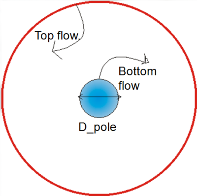
The temperature forcing wants to bring warm water inwards in our experiment (warm air/water polewards in the real atmosphere/ocean) and cold water outwards (equatorwards). For low rotation rates (small f), the Rossby radius is much larger than the circumference of our tank (a latitudinal circle in the atmosphere). In this case, the circulation is symmetric with respect to the pole and cold fluid flows inward on the bottom and gets deflected to the right resulting in anti-cyclonic motion. Warm fluid moves outward on the top, gets deflected to the right and results in cyclonic motion. This circulation is analogous to the Hadley circulation in the low latitude atmosphere. A sketch of the deviation of the moving fluids can be seen in the following sketch:
For an intermediate rotation rate, a wave sets up where circular symmetry is broken such that cold water can flow outward throughout the entire water column at one horizontal location and warm water can flow inward at another horizontal location. For small wavenumbers (the number of wavelengths fitting into a circle), these waves are called planetary waves and are analogous to the mid-latitude atmospheric circulation. In order to get this regime, it is important that the Rossby radius of deformation has a similar scale as the circumference of the tank in the laboratory or a latitudinal circle in the atmosphere. Note that both the Hadley regime and the planetary wave regime depend on a circularly closed domain and can therefore not occur in the ocean.
For high rotation rates, the situation is more analgous to the ocean and the high-latitude atmosphere where the Rossby radius is much smaller than the ocean basin diameter (a latitudinal circle in the atmosphere). This regime is called geostrophic turbulence and we expect to see small circular vortices.
Experimental Setup
You can find our experimental setup description here: Experimental Setup for General Circulation Experiment (Wilken & Julian)
Hadley Regime f=0.1s^-1
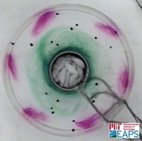
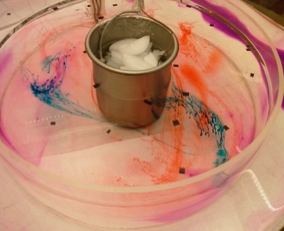
We have used a rotation rate of f=0.1s^-1. Here we present a top view onto our experiment. Turn on your computer's volume as we have commented the video!
 http://www.youtube.com/watch?v=olKFj6g-nPw&feature=channel&fmt=18
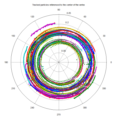
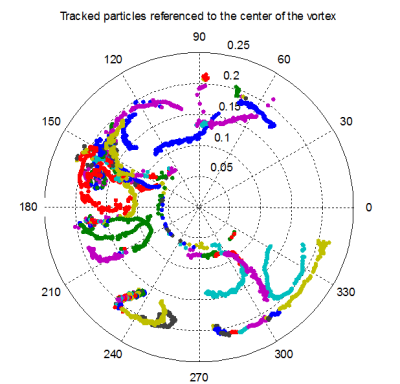
You have probably noticed the black particles flowing at the surface of the water. Previously we had developed a particle tracking software that you can find at http://mit.edu/~wilken/www/Particle_Tracker/. The program runs in Matlab and you are welcome to use it! It gives you a matrix with the positions of the black particles you can see in the video as a function of time. The results of the particle tracking for the Hadley regime shows nice, almost circular tracks, which spiral inward just a bit - as you would expect:
In our temperature record, we saw no time dependent fluctuations at all indicating that the motion is steady.
There is significant shear in the flow with cyclonic motion in the bottom and anticyclonic motion on the top as you can see in this video:
 http://www.youtube.com/watch?v=HbhpaUYgM2A&feature=channel&fmt=22
Later we have thrown a piece of permanganate which releases tracer over time close to the outside wall. As you can see the tracer only spreads up the wall and not along the bottom as would be expected from the cold water moving out on the bottom and then being warmed at the outer wall and moving up there:
 http://www.youtube.com/watch?v=JjS4TfqmK7M&feature=channel&fmt=18
Planetary Wave Regime f=0.3s^-1
In order to see planetary waves, we have really slowly increase our rotation rate until we were at f=0.22s^-1. Here we observed a wave with the wavelength equal to the circumference of the tank. This is what we call k=1.
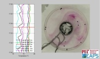
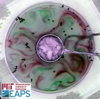
We slightly increased the rotation rate to f=0.3s^-1 where we observed a wave with two wavelengths fitting around the circumference: k=2. This means, the shape is one elongated ellipse with two points of the jet close to the cold can and two points of the jet close to the warm outside wall. We show you a video where you see the top view down onto the tank on the right and on the left you see the temperature evolution. The horizontal red bar indicates the current time. Look out for the correlation between jet location and temperature anomalies!
 http://www.youtube.com/watch?v=PcDdCdJuHI4&fmt=18&feature=channel
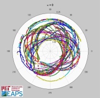
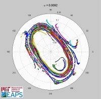
As you can see in the video, there is an angular phase propagation of the jet. This becomes more obvious on the particle tracks. Without any correction for the phase, you just see a big mess as on the left figure. However correcting for an angular phase speed of 0.093s^-1, you can really see the elongated ellipse as in the figure on the right. The video shows you corrections for subsequently larger angular phase speeds.
http://www.youtube.com/watch?v=Jc6iIE08e0E&feature=channel&fmt=18
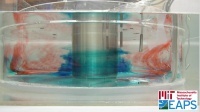
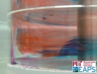
The planetary wave regime is also a strongly baroclinic flow as you can see in this image where dye streaks at different depth (i.e. colors) are almost perpendicular to each other.
Turbulent Regime f=1s^-1
Then we increased the rotation rate significantly to f=1s^-1. With an estimated Rossby radius of 2.5cm, we expect really small scale geostrophic turbulence. This can be seen in this video with small vortices present.
 http://www.youtube.com/watch?v=iFK8l3RNpfE&feature=channel&fmt=18
Here you can see the particle tracks showing nice votices with a small radius on the order of a few cm:
This is a great experiment, and it doesn't take too much preparation. You should try it!
Wilken-Jon von Appen (wilken (at) mit (dot) edu) and Julian J Schanze (schanze (at) mit (dot) edu)