...
This relationship relates the fluid horizontal speed in the tank to the tank’s rotation rate and temperature gradient. By plugging in the calculated value for the 

where u(z1) is the average velocity of a particle traveling on the surface of the water (8.5E-2 m/s for this experiment), u(z2) is the average velocity of a particle traveling near the bottom of the tank (assumed to be roughly 0), and Δz is the depth of water in the tank, here roughly 10cm. Plugging in these values, we find that the expected velocity of a particle traveling at the surface of the tank is:
...
We next plotted the zonally averaged potential temperatures calculated using the expression we previously derived in our studies of fronts and convection:

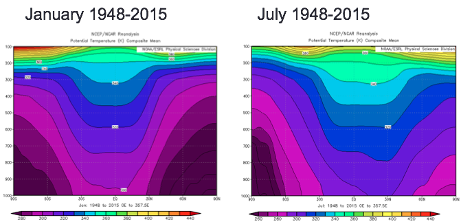
Again we observe steeper temperature gradients in the Northern Hemisphere in January and in the Southern Hemisphere in July. Note that potential temperatures over the equatorial region are relatively constant, because there is more moisture in the air above the warmer equatorial regions, according to the Clausius-Clapeyron relation. Above the 200mb height, the shape of the isotherm curves reverses direction, because this is where the stratosphere begins.
Next, we plotted the zonally averaged zonal winds:

Here we observe zonal winds increasing in velocity with height. The strongest thermal winds are located above around 30ºN and 30ºS, where the temperature gradients are strongest. Again, the winds are stronger in the winter.
The correlation between the zonal winds and the temperature gradient are more easily observed when overlaying the two data plots:

To further reiterate the relationship between the winds and the temperature gradient, we can recall the expression for thermal wind we derived in our study of fronts in terms of temperature and in pressure coordinates:

We calculate the left hand side (LHS) and right hand side (RHS) of the expression at 30ºN in January and 30ºS in July where and when the zonal winds are strongest using the data from the zonally averaged plots above. The following values were used:

From the above calculations, we see that the the LHS and RHS for both January 30ºN and July 30ºS agree well, showing that the atmosphere obeys the thermal wind relation. We next plotted the zonally averaged vertical winds, given by the formula:

Where w is negative, the air is rising.

In January, we observe air strongly rising over the equator and strongly sinking around 30ºN. In July, we observe air strongly rising over the equator and strongly sinking around 30ºS. Near the surface in both January and July, the maximums in upward vertical velocity are shifted slightly north of the equator, likely because the Northern Hemisphere has more land, which heats faster than water.
We next plotted the zonally averaged meridional winds where positive values correspond to northward moving winds:

In the January plot, high altitude winds move toward the North Pole from the equator to around 30ºN and low altitude winds move from 30ºN to the equator. The opposite pattern is observed in July.
Combining the vertical, meridional, and zonal wind data helps visualize the Hadley Cell circulation in the atmosphere. Here the meridional wind data is plotted over the vertical wind data, with the zonal components marked:

These plots show the Hadley Cell circulation in the Northern Hemisphere in January and in the Southern Hemisphere in July. We see similar but opposition motions between the two hemispheres.
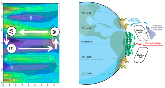
Comparing the overlaid plot of meridional and vertical wind in January with the cartoon shown above we can think about the moisture in the atmosphere. Following the Clausius-Clapeyron relationship, the warm air around the equator is also moist. As this warm moist air rises above the equator, it cools adiabatically and the moisture condenses out of the air, creating precipitation and rainforests in equatorial regions. The air high in the atmosphere follows the Hadley Cell moving to around 30ºN. As the air descends over 30ºN, it adiabatically warms. However, this air is now dry since the moisture was condensed out earlier. Therefore this descent of warm dry air results in many dry desert regions around 30ºN and 30ºS around the world.
...
Source: http://visibleearth.nasa.gov/view.php?id=56236
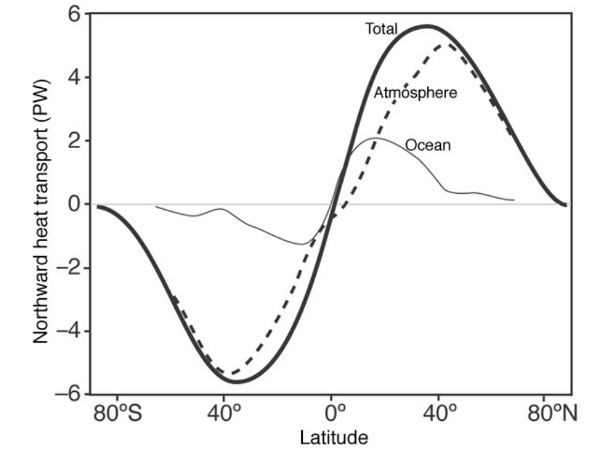
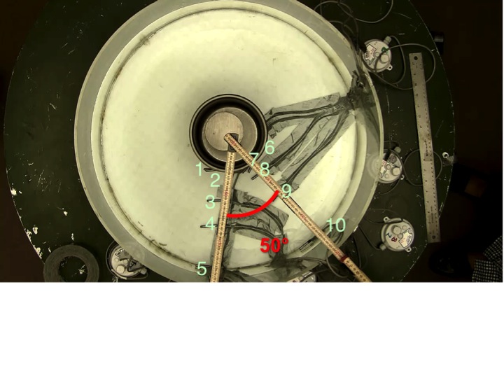
The midlatitude eddy circulation, which we can observe surrounding the pole in the satellite image above, is important for heat transport in the atmosphere. Eddies occur at higher latitudes than the Hadley Cells and as the plot above shows, estimates as in the plot above show, are responsible for most of the heat transport required by the differential heating of the Earth. Once again we used a tank experiment and atmospheric data to study these eddies. Since eddies occur in the midlatitudes, the Earth’s rotation more strongly affects motions in these eddies than the Hadley Cell motions near the equator. Therefore, to mimic eddies in our tank experiment, we used a high rotation rate and temperature gradient. To study eddies in the atmosphere, we used atmospheric data to study the heat transport involved in the midlatitude eddies.
From the figure above, detailing heat transport by latitude, heat transport is at a maximum near 40ºN and S, where eddies occur. We integrate the zonally averaged heat flux due to eddies, to find the net poleward heat flux using the following equation,

where a is the Earth’s radius, is the latitude, cp is the specific heat, g is gravity, and [v'T'] is the zonal average of v'T' =vT-v T, with v referring to meridional wind and T referring to temperature. We will then compare its result to the figure above.
...

...
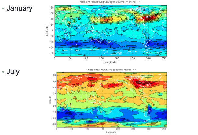

We can notice a couple interesting things from these plots. In the January when the Northern Hemisphere is experiencing winter, we see two clear maximums of Northward heat flux. These could be because the temperature gradient is strongest during the winter. The maximums are located on coasts where there are strong land-sea interactions. The combination of the stronger gradient and land-sea interaction could result in more synoptic scale storms and more eddies, resulting in stronger heat flux in those regions. In July when the Northern Hemisphere is experiencing summer, we observe that the northward heat flux is stronger overall in the Northern Hemisphere as well as more uniform. In both January and July, we see strong southward heat flux in the Southern Hemisphere.
We next plotted the zonally averaged transient heat flux, averaged over the longitudes following:

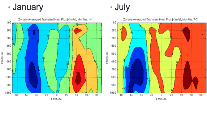
These two plots again show poleward heat flux in both hemispheres. Both plots also show two maximums of heat flux, one at a higher and one at a lower altitude. Maximums in heat flux can be caused by either differences in velocity or in temperature. Higher in the atmosphere, the heat flux maximum could be driven by the strong velocity difference around the fast polar jet. Lower in the atmosphere, the heat flux maximum could be caused by the difference in temperature between the land and ocean.
Finally, we vertically integrate the zonally averaged transient heat flux and multiply by some constants to find the zonally and vertically integrated transient sensible energy flux using:

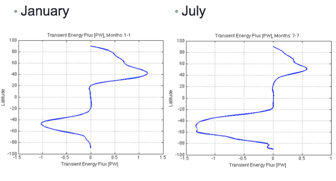
The maximum energy flux away is approximately 1PW and found around 40ºN and 40ºS because the eddy heat transport carries heat from the midlatitudes to the poles. The maximum energy flux from the atmosphere is actually about 4 PW in both North and South directions from around 40ºN and 40ºS. There is a discrepancy because we only calculated the sensible heat energy flux, neglecting the contributions from latent heat energy and potential energy that contribute to the 4PW plot.