| Section |
|---|
| Column |
|---|
| | Panel |
|---|
| title | Common Case Information: | Overview |
|---|
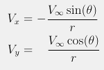
| This circle boundary layer case demonstrates the method of manufactured solutions in which an analytical heat source is derived from an analytical expression of the thermal boundary layer. This derived heat source is applied to a vortex flow around a circular annulus of radius r = [ 1 , 2 ], and the numerical heat flux at the inner boundary is checked with the analytical heat flux to a specified tolerance. All boundary temperatures are set to the analytical thermal boundary layer solution, and the initial condition is set to 1. |
|
| Column |
|---|
| | Panel |
|---|
| title | Temperature Distribution: |
|---|
|  Image Added Image Added
Note that the singularity at (θ=0) is disregarded. |
|
|
- Solution Order = 2 (non-adaptive)
- Heat Flux Adjoint Residual (Mesh Adaptive Case)
adaptation
- Solution Order =1
- Adaptation Iterations = 2
- Adaptation Method = Fixed Fraction
- Output Adapted = Heat Flux
- Anisotropy Method = Hessian
results or convergence
- Both cases reach tolerances in 2 iterations
- Compared to truth files with tolerance of
- tol: e-12
- Adapt tol : e-10
Case Details
Scalar2d_CircleBoundaryLayer
Scalar2d_CircleBoundaryLayer_Adapt
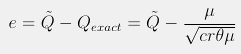
-
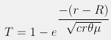 Image Added Image Added
where
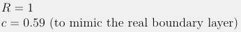 Image Added Image Added
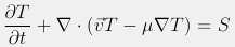
- Derived Heat Source:
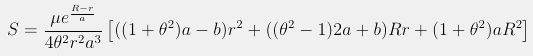 Image Added Image Added
where
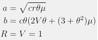 Image Added Image Added
- Non-dimensional viscosity:
 Image Added Image Added
|
|
|
Case Specific Details
| Section |
|---|
| Column |
|---|
| | Panel |
|---|
| title | Case 1 (Non-Adaptive): |
|---|
| - Solution Order: 2
- Iterations to solve: 2
- All outputs tested to a tolerance of 10-12
Job File:
Scalar2d_CircleBoundaryLayer |
|
| Column |
|---|
| | Panel |
|---|
|  Image Added Image Added
|
|
|
| Section |
|---|
| Column |
|---|
| | Panel |
|---|
| - Solution Order = 1
- Additional tested outputs: Heat flux adjoint residual
- Adaptation parameters:
- Adaptation Iterations: 2
- Adaptation Method: Fixed fraction
- Output Adapted: Heat flux
- Anisotropy Method: Hessian
- Iterations to solve on each mesh: 2
- All outputs tested to a tolerance of 10-10
Job File:
Scalar2d_CircleBoundaryLayer_Adapt |
|
| Column |
|---|
| | Panel |
|---|
| title | Case 2 Adapted Meshes: |
|---|
|  Image Added Image Added
 Image Added Image Added
|
|
|
...