...
Approach: The One-Dimensional Motion with Constant Velocity gives as an alternate representation the fact that a constant velocity can be represented as the slope of a linear position versus time graph. The graph we are given in the problem introduction is not linear overall, but it can be split into linear segments, as denoted by the different colors in the version given here:
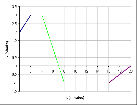
Without actually doing the math to find the slopes of each segment, we can compare them. First, it is clear that the slopes of the red section and the brown section (the 2nd and 4th segments) are both zero (the lines are horizontal). Thus, the speed of the student is zero in those segments. Another way to see the same thing is to note that from t = 2 min until t = 4 min, the students position is x = + 3 blocks, meaning the student is spending those two minutes in the library (not moving). Similarly, from t = 8 min until t = 16 min, the student is in the cafeteria.
Comparing the slopes of the other sections (blue, green and purple; or 1st, 3rd and 5th) we see that the purple (5th) section has the slope with the smallest magnitude and the green (3rd) section has the steepest slope. Thus, we expect that the student's speed (when actually moving) is slowest in the purple (5th) section, and greatest in the green (3rd) section.
With this information in hand, we can summarize the graph:
The student begins the trip in the physics building. The student leaves the physics building and walks east at a moderate pace until reaching the library. The student remains at the library for two minutes, and then hurries west to the cafeteria. The student remains in the cafeteria for 8 minutes, and then walks at a leisurely pace to the dorm, where the trip ends.
Part B
Plot the student's velocity as a function of time for the trip.