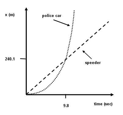
A speeder driving with a constant speed of 24.5 m/s approaches a (hidden) stationary police car on a long, straight road. The police officer detects the speeder using radar, and so the instant the speeder passes the police car, it begins accelerating after the speeder at a rate of 5.00 m/s2. How long will it take for the police car to catch up to the speeder from the instant its acceleration begins?
There are two separate systems here. Both the police car and the speeder's car will be treated as point particles.
The police car experiences a constant acceleration as a result of the action of the pavement against its wheels.
The motion of the speeder's car will be modeled as One-Dimensional Motion with Constant Velocity. The motion of the police car will be modeled as One-Dimensional Motion with Constant Acceleration.
We will write an expression for the position of each vehicle as a function of time and then set the positions equal to each other. Since we have the freedom to pick our coordinate system, we can help ourselves in this problem by choosing the positive direction to be the direction of motion and setting x = 0 and t=0 at the point when the speeder passes the police car.
The appropriate Law of Change for the speeder is:
Unknown macro: {latex}
\begin
Unknown macro: {large}
[x_
Unknown macro: {rm sp}
= x_
Unknown macro: {rm sp,i}
+ v_
t ] \end
where the subscript "sp" stands for "speeder".
The appropriate Law of Change for the police car is:
Unknown macro: {latex}
\begin
Unknown macro: {large}
[ x_
Unknown macro: {rm pc}
= x_
Unknown macro: {rm pc,i} + v_
t + \frac
Unknown macro: {1}
Unknown macro: {2}
a_
t^
Unknown macro: {2}
]\end
where "pc" stands for "police car".
Before setting these equations equal to each other, it is a good idea to substitute the zeros so that we can cancel some of the many terms. In this problem, we have chosen our axis in such a way as to make xsp,i = xpc,i = 0. We also know that vpc,i = 0 because the police car was at rest before the speeder passed it.
Doing this and setting xsp = xpc gives:
Unknown macro: {latex}
\begin
Unknown macro: {large}
[ v_
Unknown macro: {rm sp}
t = \frac
Unknown macro: {1}
Unknown macro: {2}
a_
Unknown macro: {rm pc}
t^
] \end
This is actually a quadratic equation in t, except that the constant term is absent. To be clear, we can rearrange:
Unknown macro: {latex}
\begin
Unknown macro: {large}
[ \frac
Unknown macro: {1}
Unknown macro: {2}
a_
Unknown macro: {rm pc}
t^
- v_
Unknown macro: {rm sp}
t = 0 ] \end
This equation has two roots, which are easily obtained by factoring:
Unknown macro: {latex}
\begin
Unknown macro: {large}
[ t_1 = 0] [ t_
Unknown macro: {2}
= \frac{2 v_{\rm sp}}{a_{\rm pc}} ] \end
We select the second root, since we are interested in the time that the police car catches up to the speeder, not the time that the speeder passes the police car. Thus, we find:
Unknown macro: {latex}
\begin
Unknown macro: {large}
[ t = \frac{2 v_{\rm sp}}{a_{\rm pc}} = 9.8\;
Unknown macro: {rm s}
] \end
One way to help visualize the situation is the plot separately the position of the speeder and of the police car on the same graph of position vs. time
Unknown macro: {latex}
\begin
Unknown macro: {large}
[x_
Unknown macro: {rm sp} = v_
t]\end
Unknown macro: {latex}
\begin
Unknown macro: {large}
[x_
Unknown macro: {rm pv}
=\frac
Unknown macro: {1}
Unknown macro: {2}
a_
Unknown macro: {rm pc}
t^2]\end


