Concession: I could not figure out how to change the font size for the Wiki Page and thus I apologize if my image captions are difficult to spot.
I will research the 2010 eruption of the Icelandic volcano Eyjafjallajokull in order to simulate its ash dispersal using HYSPLIT. By simulating the ash dispersal during different times of the year I hope to determine how the ash dispersal varies with different atmospheric circulation patterns–both by season and by week.
Eyjafjallajokull Background Info
| Country | Latitude | Longitude | Elevation | Eruption Date | VEI (0-7) | Erupted Material Mass |
|---|---|---|---|---|---|---|
| Iceland | 63.633 degrees North | 19.633 degrees West | 1651 m | April 14, 2010 | 3 | 4.8±1.2·10^11 kg |
Despite its moderate ranking on the VEI (Volcanic Explosively Index) given its max plume height and magma discharge, Eyjafjallajokull caused significant ash dispersal. 80% of the erupted material comprised of airborne ash, and the ash dispersed over an area of approximately 7 million km^2 in Europe and the North Atlantic. While 50% of the ash fell in Iceland, .02% reached mainland Europe.
The ash caused great trouble to Europe and led to the closure of UK airspace from April 15th through 20th, for finer ash particles clogged airplane engines.
Plume Height

Image 1: Shows the plume height of the ash from the Eyjafjallajokul eruption. The average plume height is 7.3 km (approximately 2/3rds of the height of the troposphere).
While the plume height ranged from 3 to 10 km, we will use its average plume height of 7.3 km for our simulations of Eyjafjallajokul.
Source: NASA, https://www.nasa.gov/topics/earth/features/iceland-volcano-plume-archive1.html
Ash Dispersal

Image 2: Shows the ash dispersal from Eyjafjallajokul on April 19th, 2010. The ash went so far as to reach mainland Europe and cover a significant portion of the United Kingdom.
Source: NASA, https://www.nasa.gov/topics/earth/features/iceland-volcano-plume-archive1.html
HYSPLIT Simulations for Eyjafjallajokull (Varying Eruption Date)
The simulations will be computed using HYSPLIT (https://www.arl.noaa.gov/hysplit/hysplit/), a model developed by the National Oceanic and Atmospheric Administration (NOAA)'s Air Resources Laboratory. The model is used for tracer transport and computes air parcel trajectories; it is similar to ESGlobe, which we used in Project II. Its computational approach employs a combination of the Lagrangian and Eulerian methodologies. The Lagrangian approach uses a frame of reference that moves with the air parcels and the Eulerian approach uses a fixed 3D frame of reference.
Although the eruptions contributing to the majority of ash fall lasted for 6 days, the simulations will cover the first three days of eruptions.
April 14-16, 2010
First I will simulate the eruption on its actual eruption date of April 14th. I will also examine the constant pressure surface for an atmospheric pressure of 500 mb on the second day of the eruption in order to determine if the dispersal followed the expected wind patterns.
Constant Pressure Surface
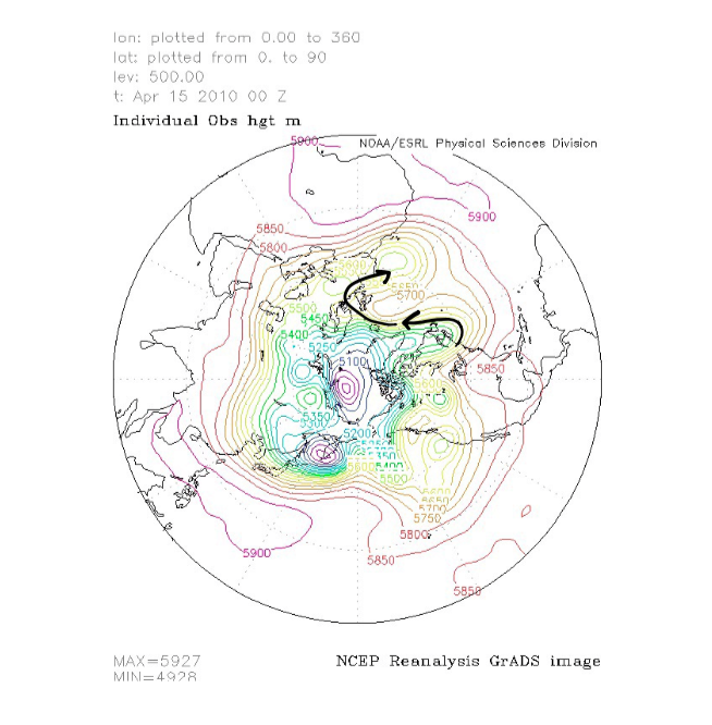
Image 3: Shows the constant pressure surface for 500 mb on the second day of the eruption. The contour lines illustrate the wind patterns for horizontal wind flows on a constant pressure surface. The coriolis force balances the pressure gradient, and thus the flow follows the constant pressure lines. Black arrows illustrate the relevant flows around Iceland. The winds move eastward towards England and then south. They also move north-westwards.
Simulation of Particle Positions for April 14-16 Eruption
Image 4: 3-day ash dispersal simulation for Eyjafjallajokull for actual eruption date of April 14, 2010. The plume initially moves north-eastward and then south-westard. The two layers closest to the Earth's surface spread the furthest.
The ash dispersal from the simulation follows the wind movements evident in the constant pressure surface graph.
Ash Dispersal by Py Plume Arrival Time for April 14-16 Eruption
Image 5: 3-day Ash dispersal by arrival time for Eyjafjallajokull for actual eruption date of April 14, 2010. The ash reaches the eastward regions.
I will now simulate the ash dispersal for if the eruption occurred a week earlier. I hope to establish a sense of the magnitude of weekly variations in ash dispersal before examining the dispersal for the eruption in different seasons.
April 7-9, 2010
Simulation of Particle Positions for April 7-9 Eruption
Image 6: 3-day ash dispersal simulation for Eyjafjallajokull for eruption date of April 7, 2010, a week earlier from its actual eruption date. The plume initially moves north-eastward and then south-westard. As the plume moves northward it deflects to the east and as it moves southward it deflects to the west as predicted by the rightward deflection of the coriolis force in the northern hemisphere. As opposed to the dispersal for the prior week, part of the northward plume is swept into the polar regime. In contrast to what we would expect from theoretical predictions, the plume in the polar region moves clockwise when due to the coriolis force in the northern hemisphere, we would have anticipated it to move counter-clockwise.
Unlike in the simulation for the eruption on its actual date of April 14th, in the simulation for the eruption a week earlier, part of the plume is swept into the polar region and causes dispersal in dramatically different regions.
Ash Dispersal by Py Plume Arrival Time for April 7-9 Eruption
Image 7: 3-day Ash dispersal by arrival time for Eyjafjallajokull for eruption date of April 7, 2010. The ash reaches Europe and encircles the north pole.
I will now simulate the eruption in January to investigate how the dispersion changes by season–specifically in the winter when the equator-pole temperature gradient peaks. I hope to determine if the variation by season exceeds that by week and if so, the patterns that characterize winter ash dispersal.
January 1-3, 2010
Simulation of Particle Positions for January 1-3 Eruption
Image 8: 3-day ash dispersal simulation for Eyjafjallajokull for eruption date of January 1-3, 2010. The plume initially moves towards the southwest and then begins to rotate anti-cyclonically (in conflict to what theory would predict about the mean flow near the north pole where the Earth's rotation has a strong influence). The southern tip of the plume laters moves southward and deflects to the east rather than to the west as the right-ward deflection from the coriolis force would predict. The plume ultimately wraps around Iceland.
Ash Dispersal by Plume Arrival Time for January 1-3 Eruption
Image 9: 3-day Ash dispersal by arrival time for Eyjafjallajokull for eruption date of January 1, 2010. The ash spreads in a circle around Iceland and reaches both the U.S. and Europe.
In order to determine if any dispersal patterns characterize the month of January or the winter months more broadly we will now look at a simulation a week later in January to look for similarities.
January 8-10, 2010
Simulation of Particle Positions for January 8-10 Eruption
Image 10: 3-day ash dispersal simulation for Eyjafjallajokull for eruption date of January 8-10, 2010. Ultimately the plume stretches around the pole in both cyclonic and anticyclonic directions.
Ash Dispersal by Plume Arrival Time for January 8-10 Eruption
Image 11: 3-day Ash dispersal by arrival time for Eyjafjallajokull for eruption date of January 8, 2010. The ash spreads both towards the northeast and towards the southeast.
The ash dispersal by plume arrival images for the eruptions from January 1-3 and from January 8-10 do not exhibit any prominent similarities–the dispersal in the first week of January forms a circle around Iceland whereas in the second week it moves only northeast and southeast in separate streams. Thus we cannot identify any large scale trends for the January dispersals.
Next I will look at simulations for the warmer month of July. I anticipate that the ash will disperse over a smaller area in July for the lower temperature gradient should result in slower zonal winds.
July 1-3, 2010
Simulation of Particle Positions for July 1-3 Eruption
Image 12: 3-day Ash dispersal by arrival time for Eyjafjallajokull for eruption date from January 1-3, 2010. The ash forms various spiraling patterns as it spreads into different regions. It may have been swept into different eddy cells.
Ash Dispersal by Plume Arrival Time for July 1-3 Eruption
Image 13: 3-day Ash dispersal by arrival time for Eyjafjallajokull for eruption date of July 1, 2010. The ash spreads north in both east and west directions. The northeastward flow also extends south in a counter-clockwise spiral.
I will now look at a simulation for the following week in July to search for larger scale dispersal trends for the month.
July 8-10, 2010
Simulation of Particle Positions for July 8-10 Eruption
Image 14: 3-day Ash dispersal by arrival time for Eyjafjallajokull for eruption date from July 8-10, 2010. The plume initially moves southeastward and then begins to spiral counter-clockwise towards the pole. The counter-clockwise motion towards the pole confirms theoretical predictions that due to the effect of the coriolis force at higher latitudes, the flow would move counter-clockwise like the Earth's rotation. In the final day, the ends of the plume deflect eastward; the ends may have been caught in eddy cells.
Ash Dispersal by Plume Arrival Time for July 8-10 Eruption
Image 15: 3-day Ash dispersal by arrival time for Eyjafjallajokull for eruption date of July 8, 2010. The ash splays northward.
Similar to those for January, the two July simulations did not demonstrate any major similarities. I did not identify any dispersal trends for July. Moreover, the areas spanned by the ash did not noticeably differ in the January versus July simulations–despite my prediction that the more extreme temperature gradient in the winter would lead to a larger covered area due to higher zonal winds.
Conclusions
By simulating Eyjafjallajokull for various eruption dates, I had sought to investigate how the circulation patterns changed both seasonally and weekly and whether the seasonal versus weakly variations dominated the ash dispersal patterns. Simulations showed that the weekly changes in atmospheric circulation patterns dominated any seasonal trends. Eyjafjallajokull sits at the boundary between two different air masses (between the polar and eddy regimes--air nearer to the poles is generally cold and dry whereas at mid-latitudes it is warmer and also influenced by the tropics). This region is influenced by the North Atlantic Oscillation (NAO) phenomenon in which the circulation patterns vary dramatically.
The pronounced weekly variation in the ash dispersal may result from the varying eddies that pass by the region of the volcano. The eddies are mesoscale (order of 1000 km), and thus which eddy occupies the region during the eruption would likely function as the main determinant of the ashes' dispersal. Moreover, the local variance has significant downstream effects. In simulation for the eruption on January 1, 2010, the ash reached the U.S. whereas in the simulation a week later on January 8, 2010, the ash reached Russia.
The simulations also give insights into our record of past volcanoes. We often research past volcanoes through the ash they deposited in Greenland ice cores. Given that in many of our simulations the ash from our Icelandic volcano did not reach its neighboring country, we may likely lack eruption recordings for many past volcanoes near Greenland.
Next Steps
My simulations did not demonstrate seasonal trends; in order to demonstrate seasonal trends, one should take the daily average of all dispersal simulations over the month of January versus the daily average over the month of July. Due to the daily variations, looking at individual days in January versus individual days in July did not show meaningful insights re seasonal trends.
It would also be interesting to look at the smallest time period over which changing the eruption date would cause the ash dispersal to vary. To do so, one must look into the time scales of the eddys in the Icelandic region. Further simulations should explore variations in dispersal from daily changes to the eruption date (as opposed to daily averages over month-long periods to see seasonal trends).