Overview

Elisa Boles and Ju Chulakadabba | May 26th, 2017

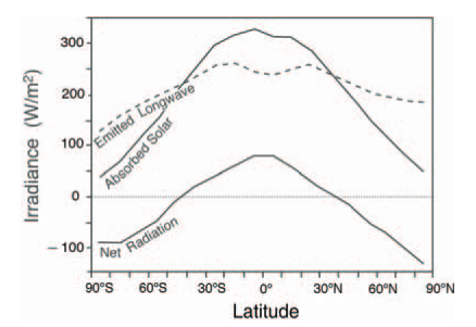
Our world is a complex system. Solar radiation hits the earth most strongly at the equator, where the sun is directly overhead. The uneven heating of the planet creates a temperature gradient between the equator and the poles. However, the emitted longwave radiation is lower in the tropics and higher at the poles than the absorbed solar, meaning that there must be a net transport of heat pole-wards (Illari & Marshall, 2010).

(Marshall & Plumb, 2008)

If we consider the earth as one big system, we find that heat transport from the equator to the poles is not performed in the same manner across all latitudes. The change in regime is largely due to the change in Coriolis parameter with latitude; near the equator, the effects of rotation are relatively minimal, but at high latitudes these become very important (Illari & Marshall, 2010). The two main regimes are the following:

1)         The Hadley Cell Circulation: the regime near the equator (~ 30N to 30S) where the solar radiation strikes the Earth relatively directly and the effects of rotation (Coriolis forces) are small.

2)         The Eddy Cell Circulation: the regime in the mid and higher latitudes where the solar radiation strikes the Earth with relatively indirect and the effects of rotation are slightly bigger.

In order to understand the two regimes in the atmosphere, we performed two experiments on rotating tanks of water, spinning at different speeds.This setup acted as an analog to the atmosphere on our rotating earth, with the cold polar region reproduced by the ice bucket. Varying the rotation rate of the tank was akin to altering the latitudinal location on the earth. We also examined real atmospheric mean and transient data to explore the general circulation patterns in the atmosphere.

Hadley

At low latitudes near the equator, atmospheric circulation is mostly axisymmetric. Warm air rises at the equator, moves to about 30ºN or south, where it then descends and returns to the equator. This circulation is called the Hadley Cell, which we will explore in more detail in this section.

Tank Experiment

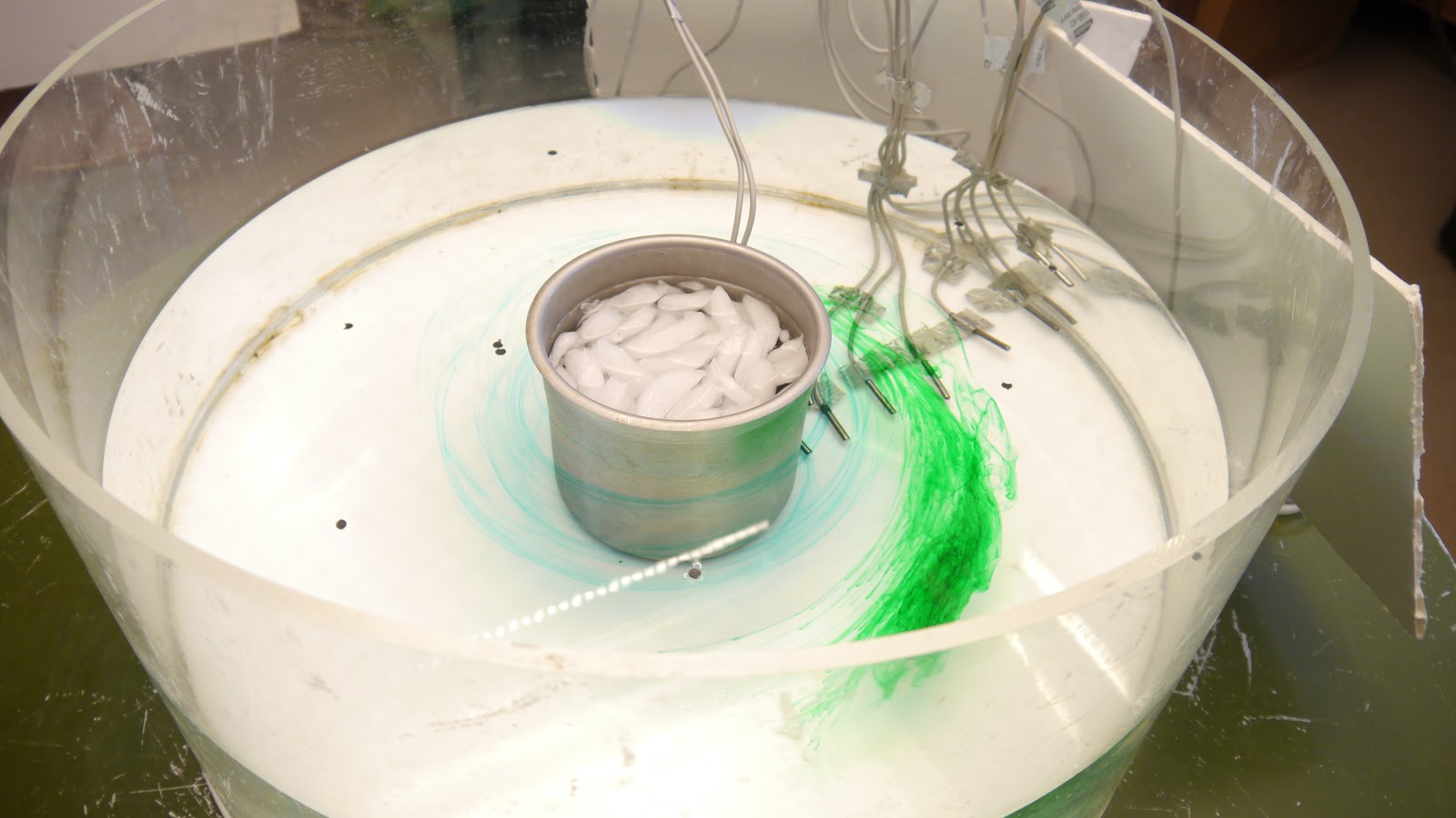
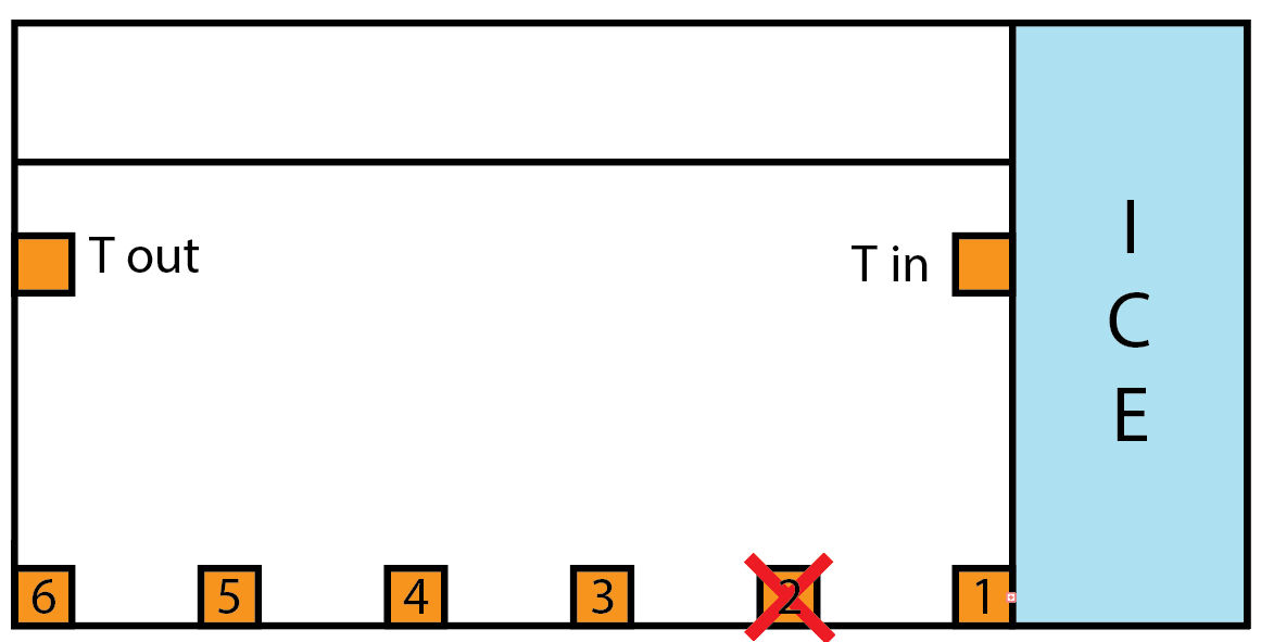
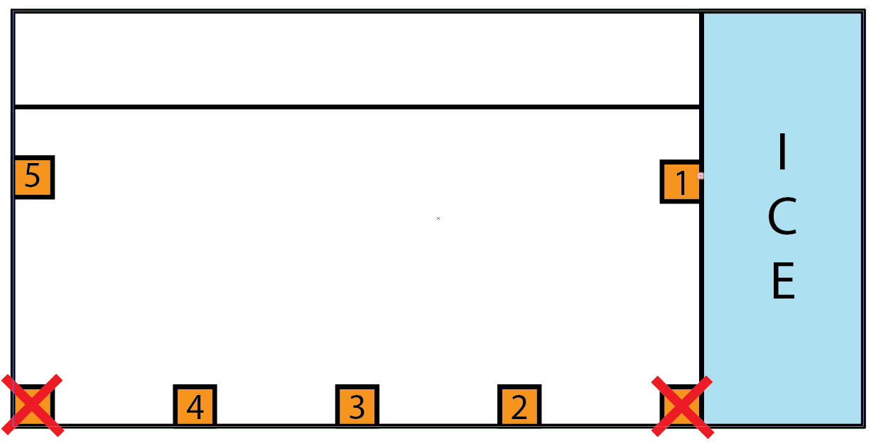
In order to imitate the circulation in the low latitudes, the first experiment was performed with a very slowly rotating tank - moving at just 1 revolution per minute. Temperature sensors were placed radially along the bottom the the tank to track the movement of heat over the course of the experiment, as well as two 10 cm above - one taped to the ice bucket and one to the edge of the larger tank. Particles were also dropped onto the water to track surface motion, and drops of dye used to visualize flows.

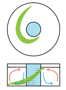
Observed from the counter-clockwise rotating reference frame, particles on the surface circled the tank, moving faster than the speed of the tank's rotation. Those towards the center of the tank were much faster than those on the outside. Dye dropped into the tank created trails that also circled the ice bucket. The dye that sank further moved more slowly and moved slightly radially outwards, while the dye that remained near the surface circled more quickly, and also moved radially inwards. These motions created a lengthening tendril of dye, which, seen from above, appeared to spiral towards the ice bucket.

 After many rotations, the spiral eventually morphed into a cone of dye around the ice bucket, just like the cone we saw in the second lab experiment. Potassium permanganate (bright purple streaks below) dropped onto the bottom of the tank also revealed the flows at depth. The dye created streaks that spread radially outwards and clockwise (counter the direction of rotation).

This behavior can be explained by radial overturning and thermal wind balance. The cold water near the tank is more dense than the warmer water at the extremities, and hence sinks and spreads along the bottom due to hydrostatic balance:

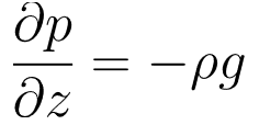
(Marshall & Plumb, 2008). This states that the vertical pressure gradient is equal to the negative of the density times the gravitational acceleration. The result of this is that the dye at the surface moved inwards, and that at the bottom moved outwards.

However, the radial temperature gradient also imposes vertical wind shear, according to the equation for thermal wind:

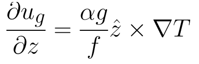
where the left hand side is the change in azimuthal velocity with height, α is the coefficient of thermal expansion, f is the coriolis parameter, and ∇T is the temperature gradient (Marshall & Plumb, 2008). In the tank, the temperature gradient then causes "winds" to develop that increase in speed with height. This is why the dye spread into long trails around the ice bucket.

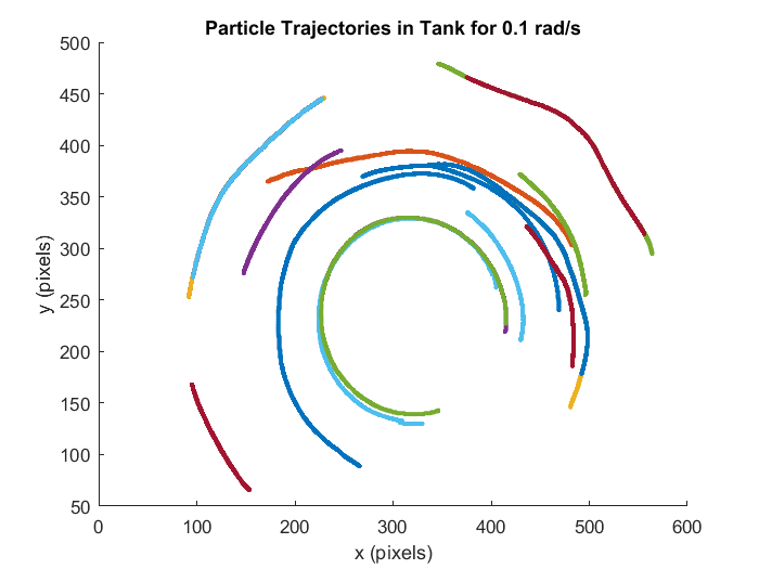
The positions of the particles at the surface could be monitored using a particle tracking software. Data showed that they followed circular paths around the center of the tank. Azimuthal velocities of the particles were calculated to be around 2 cm/s.

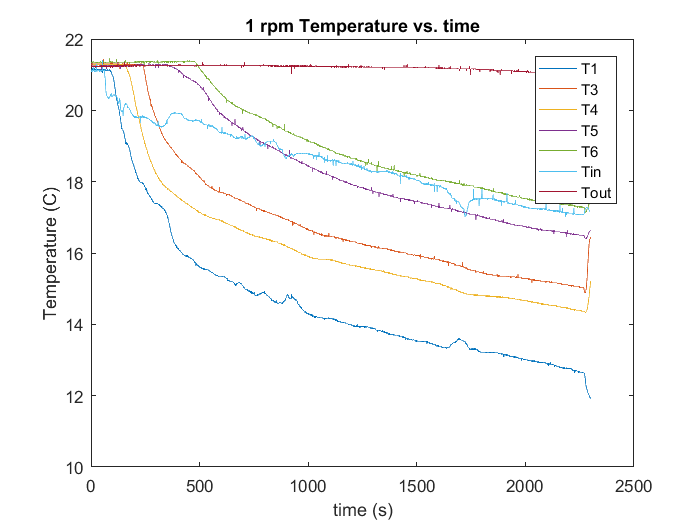
The temperature data from the thermometers revealed that an overall trend of decreasing temperature in the tank, as a result of the melting of the ice. The sensors at the bottom of the tank maintained a near-constant radial temperature over time, of about 4ºC. The temperatures higher up in the tank evolved differently however. The sensor on the edge of the tank measured a high temperature of about 21.2 ºC throughout the experiment, and the one on the ice bucket, gave a reading higher than all but the furthest sensor from the ice bucket at the bottom. These high temperatures are a result of the overturning circulation seen in the non-rotating case as well. Cold water near the ice bucket sinks and spreads along the bottom, leaving the surface water much warmer than that below.

 Discretizing the equation for thermal wind and solving for u gives

where the coriolis parameter, f, has been replaced by 2Ω, L is the radial distance between the ice bucket and the edge of the tank, and H is the height of the water (Illari & Marshall, 2010).

We can use the temperature data to calculate the right hand side of the equation, and compare it to the observed surface velocities of the paper dots.

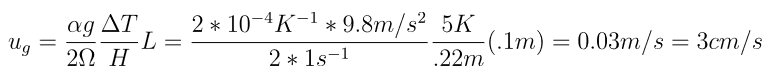
The result is close to the particle velocities found of about 2 cm/s, showing that the theory explains the observed phenomena well within margin of measurement and calculation error.

Atmospheric Data

To draw a connection from the tank experiments to the real world phenomena, we investigated monthly averages from 1948 – 2017 atmospheric data including temperature, potential temperature, and wind speed at different locations around the earth.

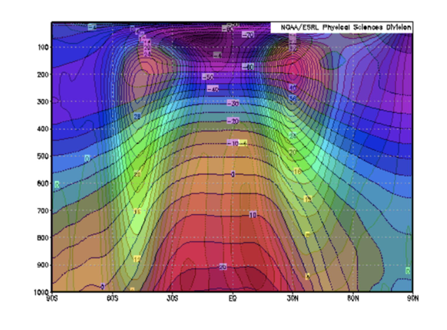
The mean horizontal temperature gradient is plotted below for all latitudes in January (left) and July (right). There is a strong horizontal temperature gradient at the surface between the equator and the poles in both cases. The gradient is especially strong in the hemisphere in which it is currently wintertime- the temperature changes faster in the northern hemisphere in January and faster in the southern hemisphere in July.  The temperature gradient decreases with latitude, and above the tropopause (about 200 mbar) in the stratosphere the gradient actually changes direction, going from coldest air over the equator and warmer air towards the poles.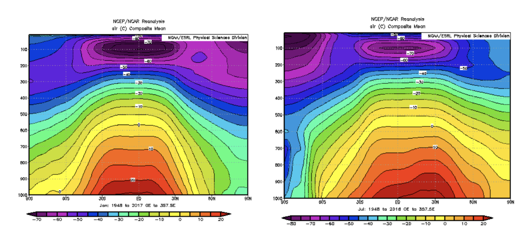

We found that the Meridional Wind, Omega (vertical velocity, in Pa/s), and Zonal Wind pattern in January differ from those in July.

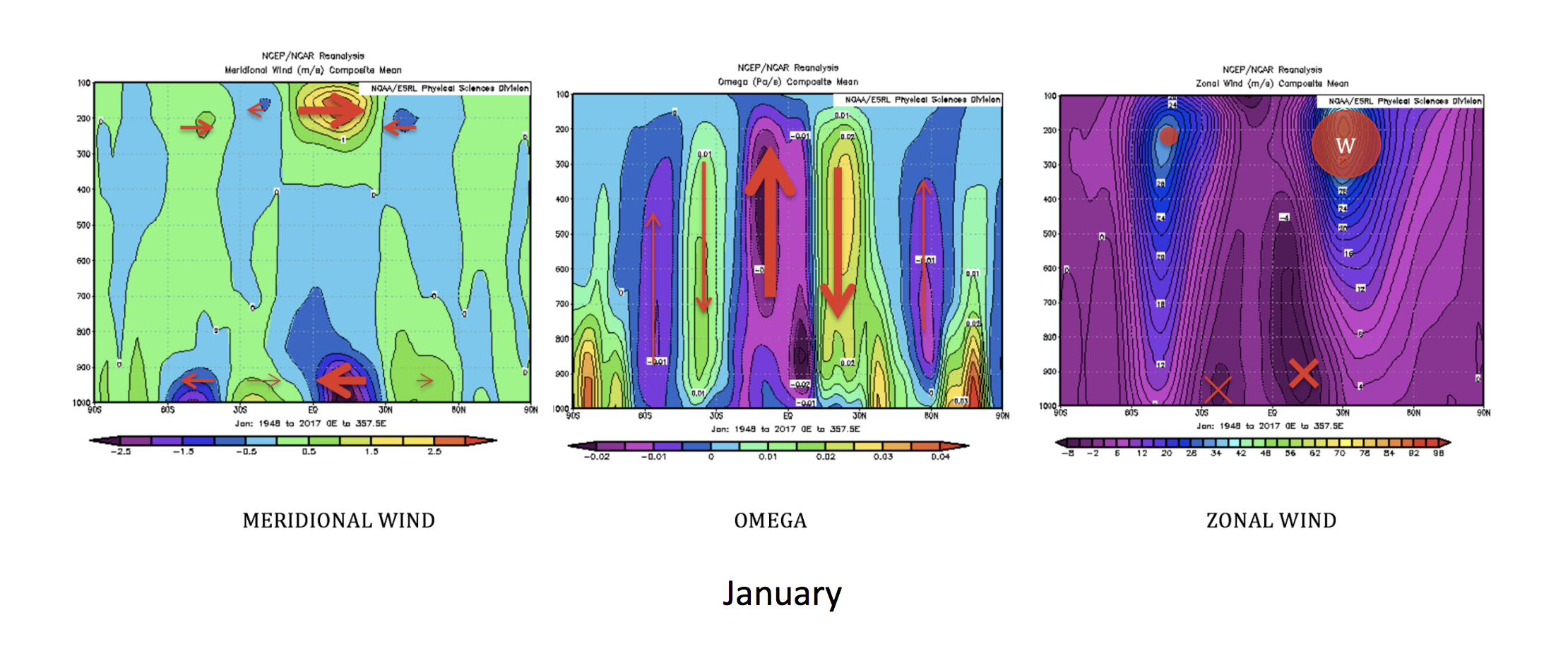
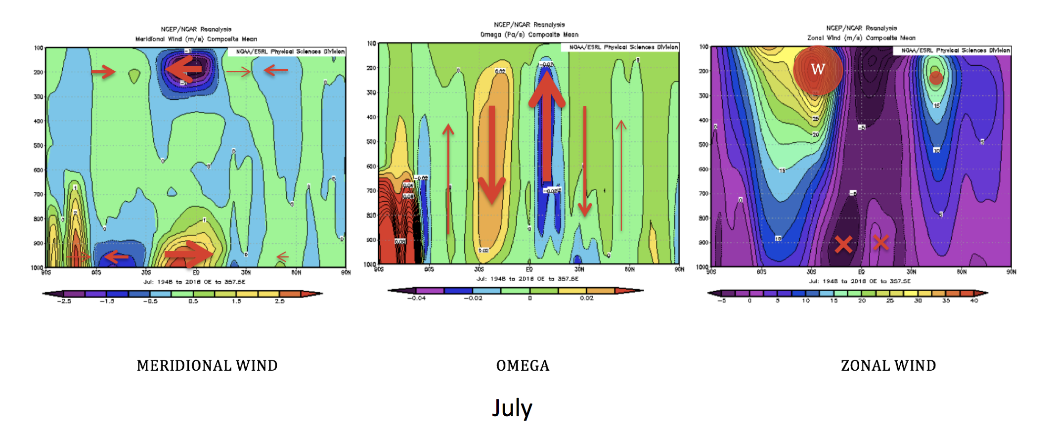
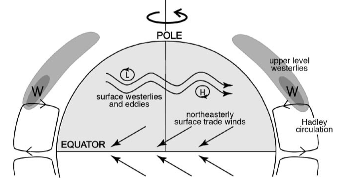
Without considering the seasons, the maximum solar heating region is near the equator since the region is almost perpendicular to the sun's radiation. This orientation creates strong rising motion of the heated air.  The flow rises and diverges toward poles.  The direction now depends on the seasons. The hemisphere in which it is wintertime has stronger temperature gradient between the equator and pole, so the flow tends to be stronger in that hemisphere. As the air moves further from the equator, it becomes closer to the Earth’s axis of rotation and starts experiencing a greater Coriolis force. The zonal velocity must increase in order to conserve the momentum of the earth system; the maximum velocity is located around 30 degrees away from the equator where the subtropical jets are located. Again, to determine the location of the maximum, we need to know the time of the year; the hemisphere that experiences winter has the strongest zonal wind. Note that the zonal wind goes from west to east near the surface and east to west high up because of the rotation of the earth.  Because of the meridional wind, the air that just rises moves meridionally towards the poles, then sinks and reverses direction, moving back to the equator. A fully completed cell is formed, the Hadley Cell.

The full schematic is captured by the figures below.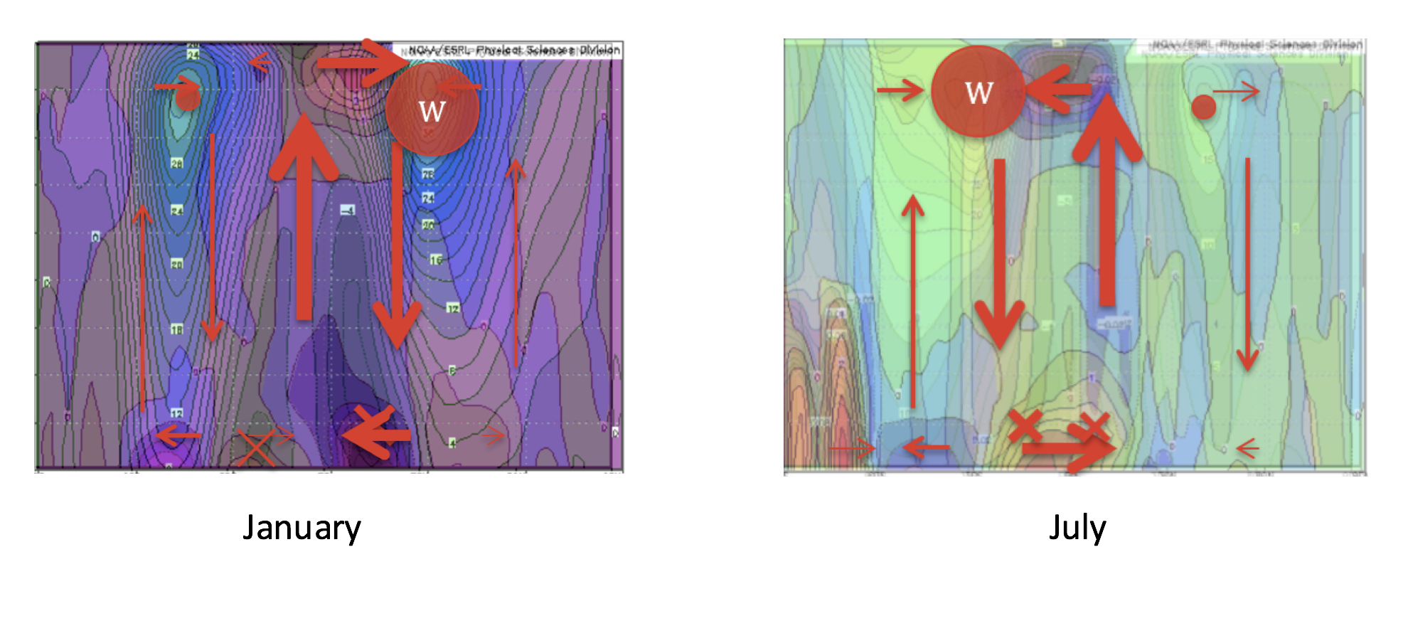

To verify the relationship between the temperature gradient and the winds (thermal wind relationship), we overlaid the figures. We found that the most abrupt temperature change regions match the edges of the Hadley cells derived from the wind data.

To verify the relationship mathematically, we plugged the values from the plot into the thermal wind equation, using the following constants:

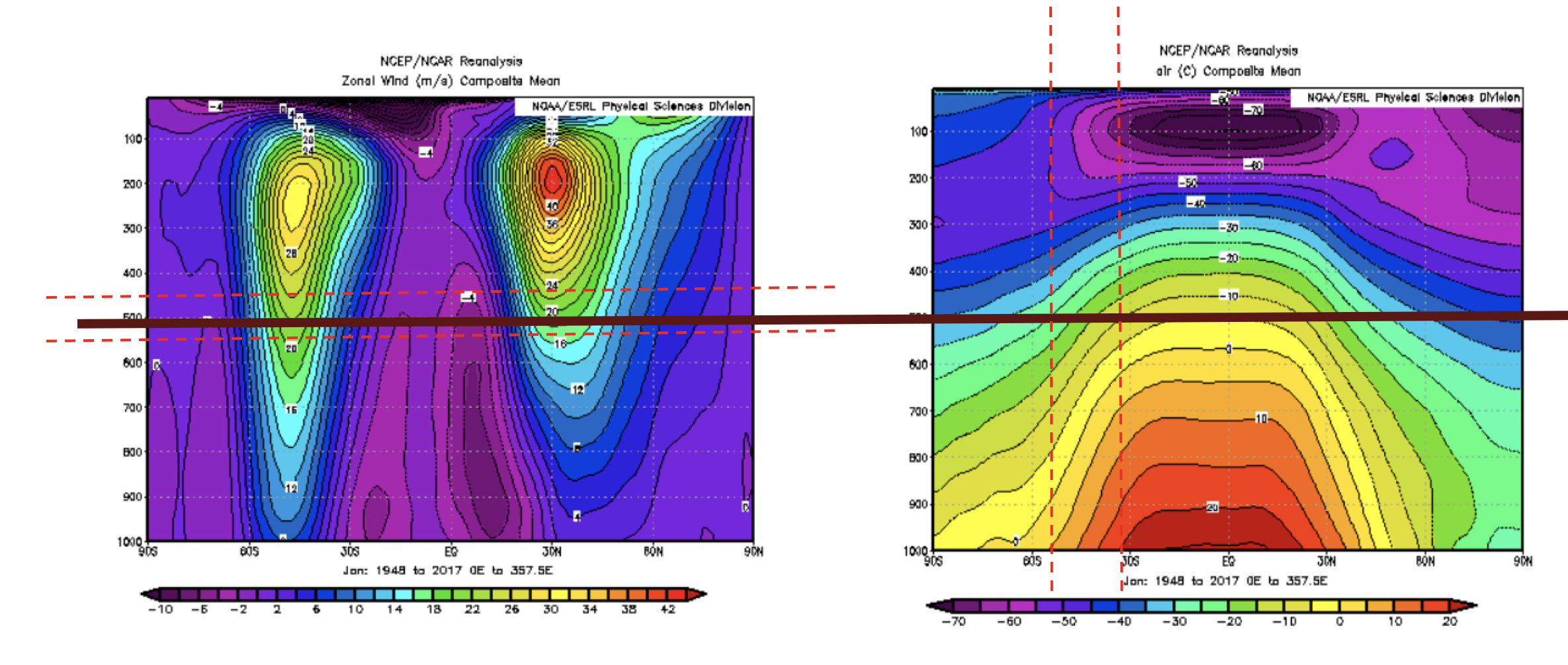
Aiming for the 500 mmb data, we can find the approximate value by using the nearby data points.

P = 450 mmb,  Zonal Wind = m/s                      Lat = -55, temp = -25 degree C

P = 650 mmb, Zonal Wind = m/s                       Lat = -35, temp = -10 degree C      

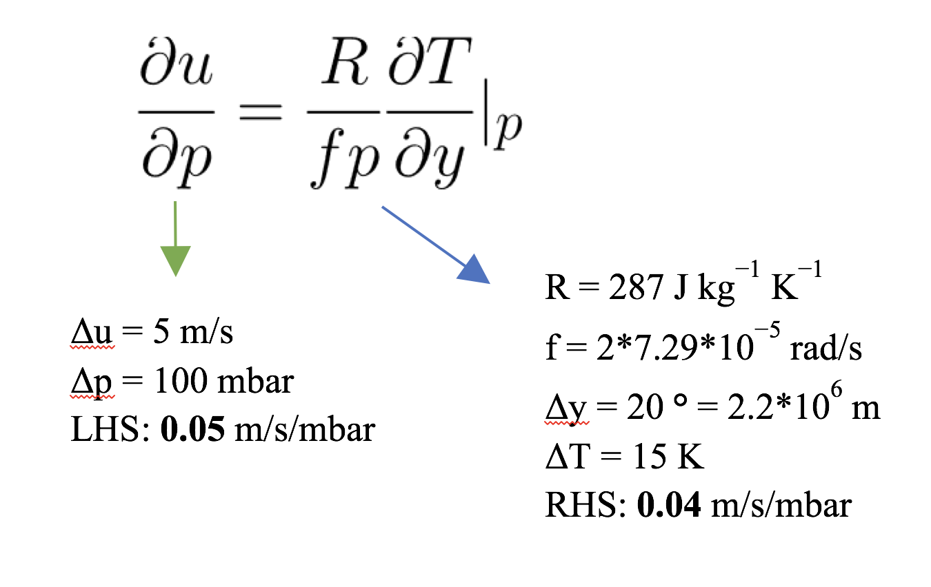
From the thermal wind equation verification, we found that both sides of the equation have the same magnitude of the results. Therefore, we can say that in both cases, the flows are in thermal wind balance.

In conclusion, Hadley cell is responsible to the heat transport in regions where the effects of rotation are small—near the equator. The Hadley cell moves warm air toward the poles and cooler the air when moving it toward the equator. The strong Hadley cell can be determined by the hemisphere experiencing winter. Additionally, Hadley cell is also in thermal wind balance.

Eddy

While the Hadley cell is critical for heat transport at low latitudes, the atmospheric mean data reveals that meridional overturning decreases significantly at higher latitudes. (There are still meridional cells, known as the Ferrel Cell and the Polar Cell, but these are weak). However, data show that pole-ward energy flux peaks beyond the edge of the Hadley cell, near 40ºN, and remains high even further towards the poles (see figure below).

(Marshall & Plumb, 2008)

The mean, zonally symmetric solution is therefore insufficient to explain the continued heat transport to high latitudes. At mid-high latitudes, potential energy that is stored in the horizontal temperature gradient can be converted to kinetic energy through the poleward transport of momentum; an increased Coriolis force results in stronger winds. Baroclinic instabilities in the flow create longitudinally asymmetric motions, which are commonly referred to as eddies.

(Marshall & Plumb, 2008)

Tank Experiment

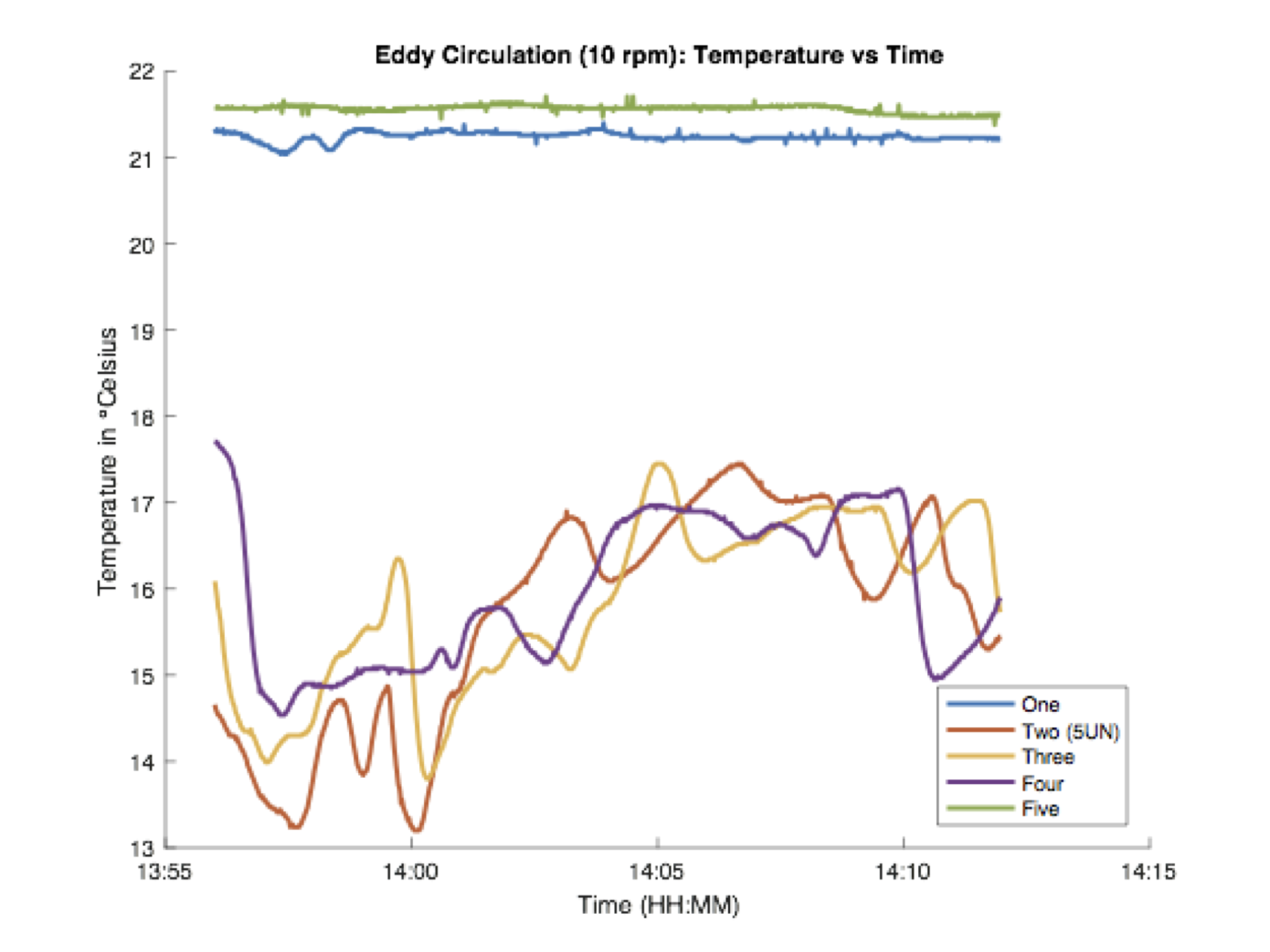
 The second experiment was, in contrast, performed at the faster rotation speed of 10 rpm in order to replicate the regime in 30N – 60N and 30S – 60S.

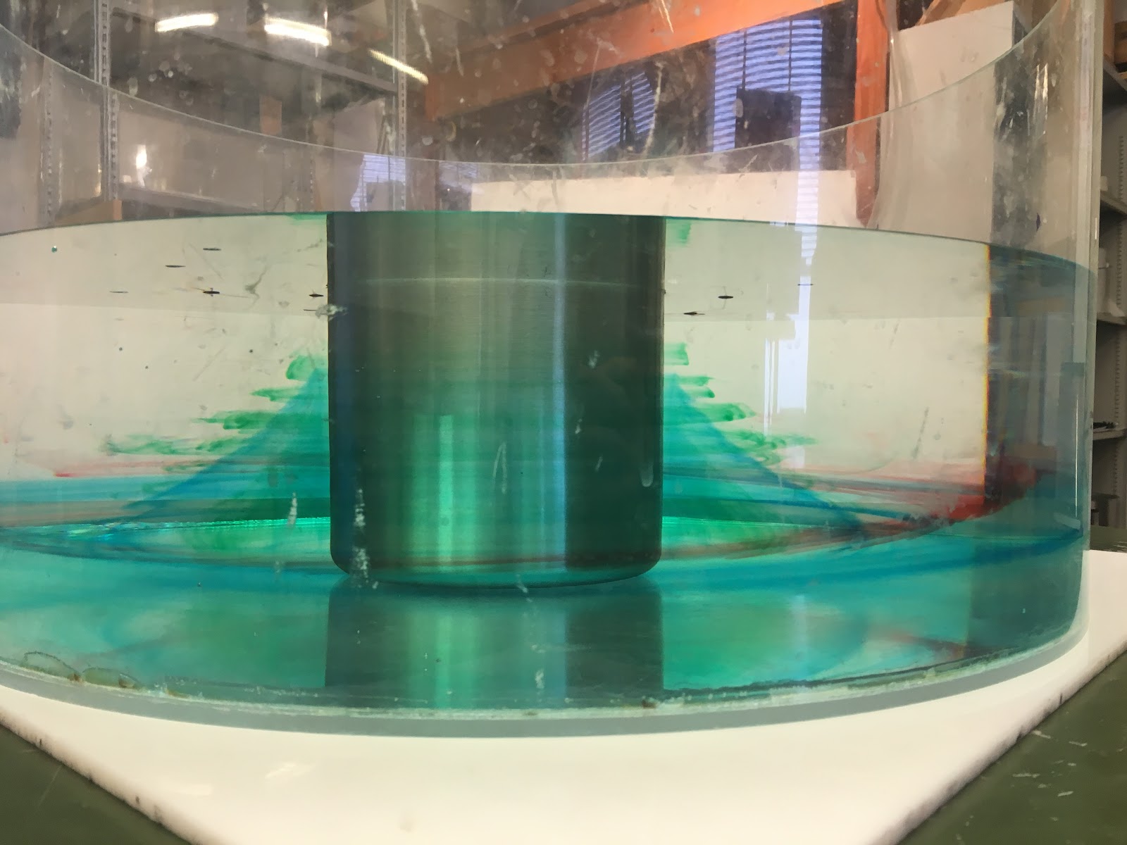
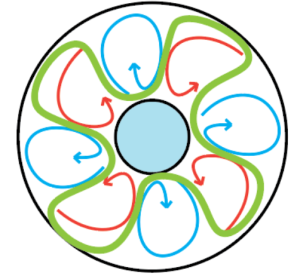
Red dye dropped near the edges and blue dye dropped near the ice bucket eventually swirled together, creating the beautiful image below. The dye helps illustrate the transport of heat through the bucket. Warm water from the outside is moved radially inwards and cold water at the center is moved radially outwards, in non-axisymmetric vortices around the tank.

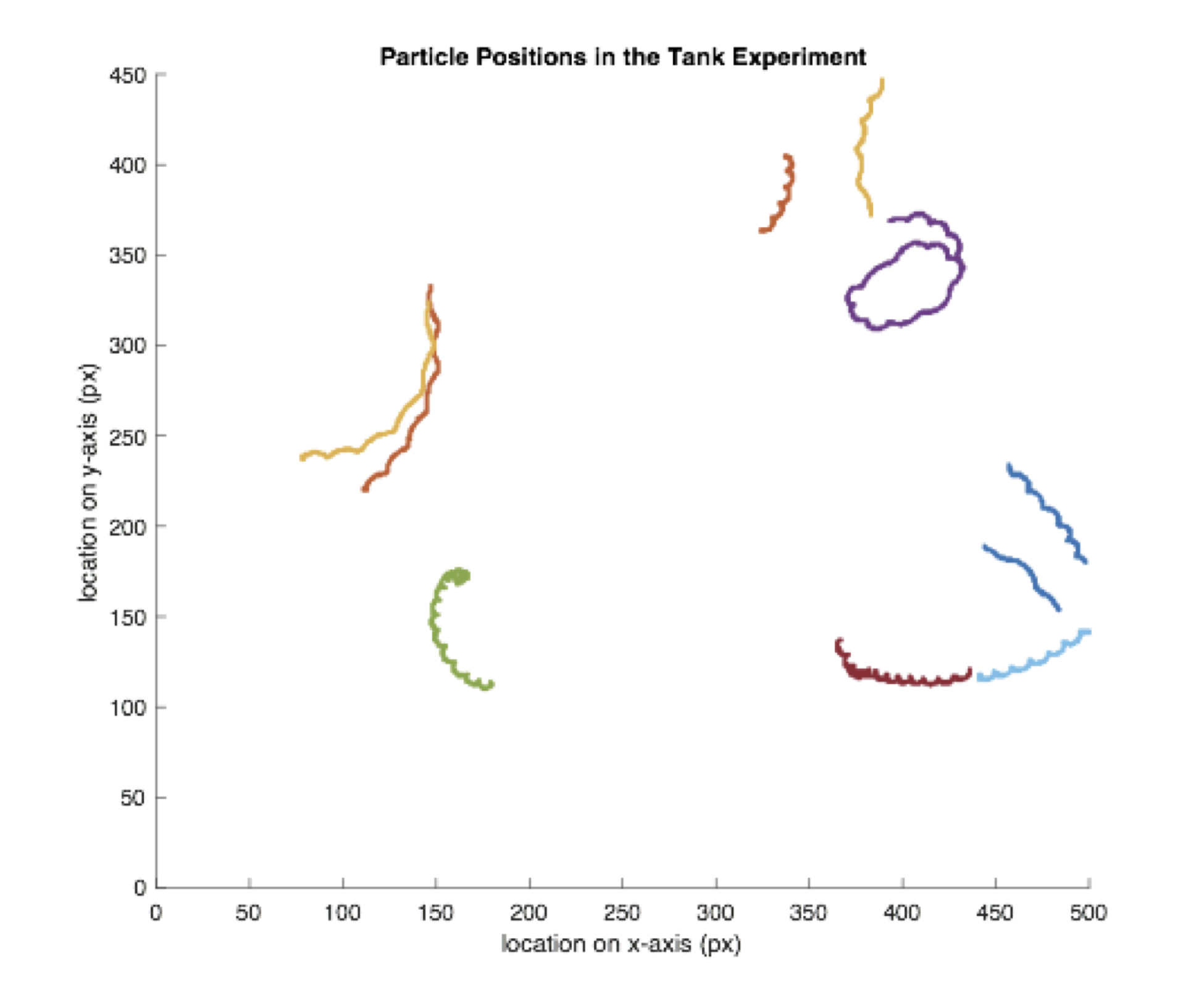
Similarly, to the first tank experiment, the particle tracker and thermometers were used to monitor the circulation and temperature in the tank. Below are plotted several particle tracks. The particles clearly do not follow the same regular, axi-symmetric motion as in the Hadley experiment.

For the temperature profiles of each sensor, we found a periodic trend of temperature, which corresponds to the observed circulation pattern: circulating from the inner part to the outer part and vice versa

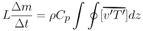
To verify the assumption that Eddy circulation plays role in transferring heat, we expect the calculated heat flux from the melt ice to be in the same magnitude as the heat flux from Eddy circulation.

We filled out parameters to the following equation.

z = 0.15 m

T’ = 1 K

ρ = 1000 kg/ m^3

Cp = 4.2 kJ/kgK

L = 333 kJ/kg

Initial Ice: 1.1 kg

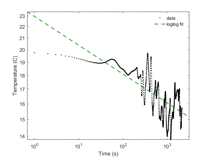
Note: To find T’, we first fit the temperature data with a log-log fit. This was chosen instead of a simple linear fit because when the Hadley temperature data is plotted in log-log coordinates the line appears linear (see below), and the eddy data seems to follow a similar downward curve.

The eddy temperature data is plotted in log-log coordinates with the corresponding fit below (left). This fit was used as the mean temperature value, T. We then subtracted this value from the raw data, which gave the figure on the right. The log-log fit seems to be a good one, because once the mean downward trend is subtracted out, the residuals remain near zero and do not exhibit further upwards or downwards trends.

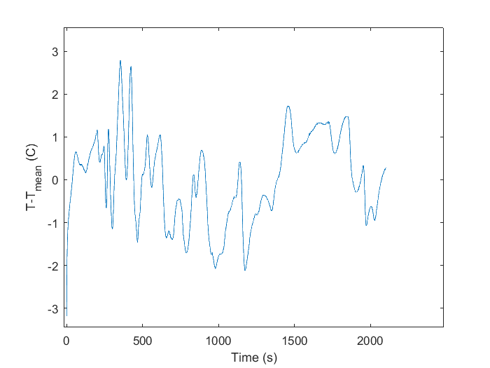
 The root mean square was then taken, such that the full calculation process can be described by:

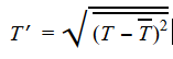
This gave a result of ~1ºC.

To find v', we find the mean of each sample track, subtract the velocity of each point with the mean, square each term, average them all, and take a square root of that average, which can be described by:

.

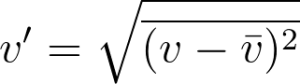This gave a result of v’ = 0.94 cm/s = 0.0094 m/s

For the left hand side, we know the latent heat fusion coefficient of the ice, mass of the initial ice, and the time the ice took to be completely melt. For the right hand side, we assume the density of the liquid to be approximately equal to that of the water. So, we know the density, specific heat of the liquid, and v’ and T’ from thermometers and particle trackers. We also need to multiply a correction factor of 0.1 to the right hand side. After plugging all the values to the heat flux equation, we find that the left hand side to be around 150 W and right hand side to be around 89 W.    

From the comparison of ice heat flux and calculated Eddy heat transport, we found that they were in almost the same magnitude—suggesting the relationship among them.

Atmospheric Data

Eddies are apparent in atmospheric potential temperature fields. The image below shows the potential temperature of the 850 mbar surface over the North Pole for a day in the winter. The swirls of the eddies between red and blue regions are particularly visible over the Pacific Ocean.

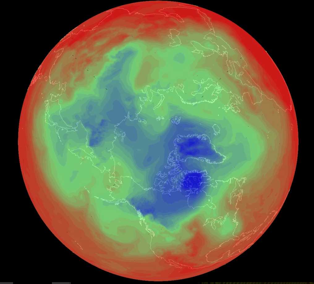
("Potential Temperature Loop", n.d.)

While atmospheric mean data could be used to study the Hadley circulation, eddies are shorter timescale phenomena and are calculated through deviations from the mean.

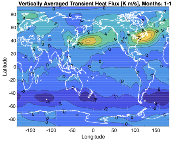
We were given data of v’t’ - the heat flux from the mean deviations for all latitudes, longitudes, and heights up to 100 mbar in the atmosphere. Looking at the vertical average of the deviations in January, we see particularly strong northward flux in regions 40ºN, over the Pacific and Atlantic Oceans. As the mean data revealed, the Hadley cell descends near 30º, with little There are also similar, though not nearly as strong, negative deviations around 40ºS as well. The values here are negative because they imply transport to the South Pole from the equator, and are not quite as large as those in the Northern Hemisphere due at least in part to the fact that the temperature gradient is larger in the northern hemisphere January, when it is winter there.

We can also plot the zonal average with height. The maximums at around 40ºN and S are evident here as well. An interesting feature is that for both latitudes, there exists a maximum near the surface, and one higher up in the atmosphere. The lower maximum, centered around 800 mbar, is a result of the large temperature gradient between the poles and equator near the surface. At higher altitudes, the temperature gradient lessens, but the meridional winds increase. The heat flux maximums near 200 mbars are a result of these stronger winds.

Finally, averaging both vertically and zonally gives the total northward flux at each latitude. Again, peaks occur just past 40 N and S. The peak in the Southern Hemisphere is very regular, while that in the northern hemisphere drops off less quickly at high latitudes. This lack of symmetry is likely a result of the fact that the majority of the continental land mass is located in the northern hemisphere, and the uneven surface leads to further atmospheric instabilities and eddies.

We can compare the results here to those summarized by Peixoto and Oort in their book, Physics of Climate. The figure below shows the total northward flux of sensible heat (not including latent heat), with breakdowns for transient eddies, stationary eddies, and mean meridional circulation. The units here are in K m/s the original units of our calculations, and winter (thin), summer (dashed) and yearly averages (thick) are plotted for each. The review here found a maximum transport for transient eddies of about 8 K m/s, twice as much as our calculations.

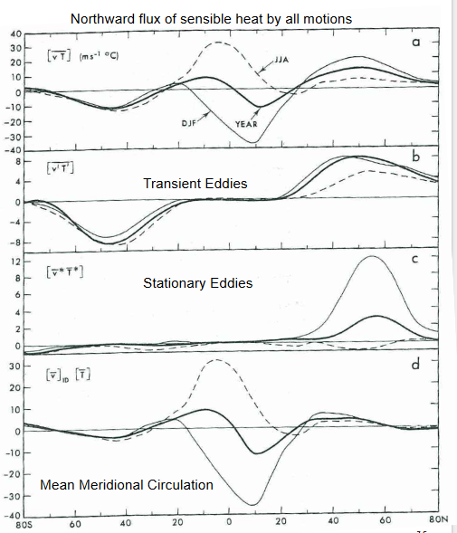
(Peixoto & Oort, 1992)

One potential contributing factor to the discrepancy is that our data has been filtered somewhat, to only account for the eddies that exist on timescales on the order of a week, but some eddies last only a couple days. There are also stationary eddies that remain relatively constant over several months, plotted in the Peixoto and Oort graph. These are especially prominent in the Northern Hemisphere during the wintertime, accounting for another 12 K m/s at 40N. Since our calculations were performed for the month of January, we can expect that the missing stationary eddy flux, if included, would improve the comparison.

The mean meridional circulation, or Hadley circulation, is also plotted, and provides a maximum of over 30 K m/s near 10ºN and S. This circulation has a much smaller effect at high latitudes however, as our mean data also showed.

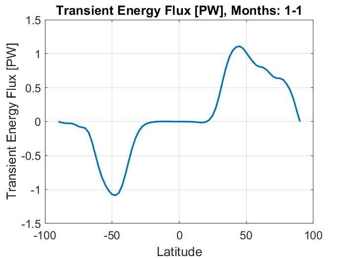
It is also useful to change the units of heat flux to Watts in order to compare our findings to the total energy flux of the earth. To do so, we vertically integrate our v’T’ zonal average and insert it into the following equation for energy flux:

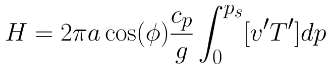
where a is the radius of the earth, ɸ is the latitude, Cp is the specific heat of air, g is gravitational acceleration. For a latitude of 40ºN, the equation gives a maximum energy flux of 1.1 PW (10^15 Watts).

This can be compared to the image below, of the total northward energy flux in the atmosphere. The ocean contributes an important part of the heat flux at low latitudes, but beyond 40N and S its transport becomes insignificant. The atmosphere

(Marshall & Plumb, 2008)

Comparing this graph to our results, we can see that it is on the same order of magnitude as the total transport of 5.5 PW at 40ºN; from our numbers, eddy transport would constitute 20% of the total at this latitude. Our results seem slightly low again however, considering that eddies are a predominant transport mechanism in mid-high latitudes. Factoring in the transient eddies and data filtration would bring us closer to the 5.5 PW, but not nearly there. The other significant method of energy transport is through latent heat, which is included in the total energy flux graph but not in our calculations. Water that evaporates near the equator and is lifted and transported pole-ward condenses, releasing latent heat and further warming the high latitudes. Including this term would likely account for most of the remaining discrepancy.

Bibliography:

Illari, L., & Marshall, J. (2010). 12.307 Project 4 General Circulation. Retrieved from http://paoc.mit.edu/12307/gencirc/climatology_lab.pdf

Marshall, J., & Plumb, R. A. (2008). Atmosphere, Ocean and Climate Dynamics: An Introductory Text. Burlington, MA: Elsevier Academic Press.

Peixoto, J.P., and A.H. Oort. (1992). Physics of Climate. United States: New York, NY (United States); American Institute of Physics.

"Potential Temperature Loop." n.d. Retrieved from http://paoc.mit.edu/labguide/images_new/850mbPotTempLOOP.gif