Introduction
The circulation of the atmosphere across the globe is chaotic; as a result, long-term weather prediction is theoretically impossible. However, large-scale structures in atmospheric circulation are stable over time and can be described by basic ideas about energy balance in the Earth system.
These constraints are explored in three other tank experiments described on this wiki: Balanced Motion, Fronts and Convection. Bringing these concepts together into a general circulation model explains the existence of some persistent features of the atmosphere, including the subtropical and polar jet streams, the trade winds, and the midlatitude bands in which rotating weather systems can be observed.
Theory
Balanced Motion
The Balanced Motion experiment develops three kinds of force balance: hydrostatic balance in the vertical, and geostrophic and cyclostrophic balance in the horizontal. It also introduces the Rossby number as a tool to determine whether geostrophic or cyclostrophic balance dominates in a given system.
Hydrostatic balance relates the pressure at a given surface to the weight of fluid above it.
| p = \rho g (H - z) |
where p is pressure, \rho is density, g is the acceleration due to gravity, H(r) is the height of the free surface, and z is height.
Geostrophic balance is between the Coriolis force and the pressure gradient force, and dominates when centrifugal force is small.
| 2 \Omega v_\theta = g \frac{\partial h}{\partial r} |
where \Omega is the component of the Earth's rotation parallel to the force of gravity, v_\theta is the azimuthal velocity, h is height and r is radius from the tank center.
Cyclostrophic balance is between centrifugal force and the pressure gradient force, and dominates when the Coriolis force is small.
| \frac{v_\theta^2}{r} = g \frac{\partial h}{\partial r} |
Whether geostrophic or cyclostrophic balance is a better approximation is determined by the Rossby number, which is simply the ratio of centrifugal to Coriolis forces in a system.
| R_O = \frac{|V_\theta|}{2 \Omega r} |
Thermal Wind
The Fronts experiment introduces temperature gradients as an important factor leading to pressure gradients. As a consequence of hydrostatic and geostrophic balance, temperature gradients cause vertical shear according to the relation
| \frac{\partial \mathbf{u}_g}{\partial z} = -\frac{\alpha g}{f} \hat{\mathbf{z}} \times \nabla T |
where \mathbf{u}_g is the speed vector, \alpha is the thermal expansivity of the fluid, f is the Coriolis parameter, and T is temperature. This expression holds only for incompressible fluids, so is valid for the tank experiment: for compressible fluids like the atmosphere, the equation can be written in pressure coordinates instead of height.
Convection
The Convection experiment introduces convection as a method of heat transport that helps balance the earth's radiative budget. Since the earth's temperature is roughly constant over time, outgoing thermal radiation must equal incoming solar radiation. The level at which radiation balances turns out to be in the upper atmosphere: below that level, convection acts to transport heat more efficiently than radiation.
Two Regimes in the Atmosphere
The three experiments develop the framework for a model of atmospheric circulation on Earth. The equator-to-pole temperature gradient creates an energy imbalance which is equalized when air moves along pressure gradients and is affected by conservation of angular momentum as it travels meridionally. These constraints produce two structural regimes visible in the atmosphere: the Hadley Cell and mid-latitude eddies.
Hadley Cell
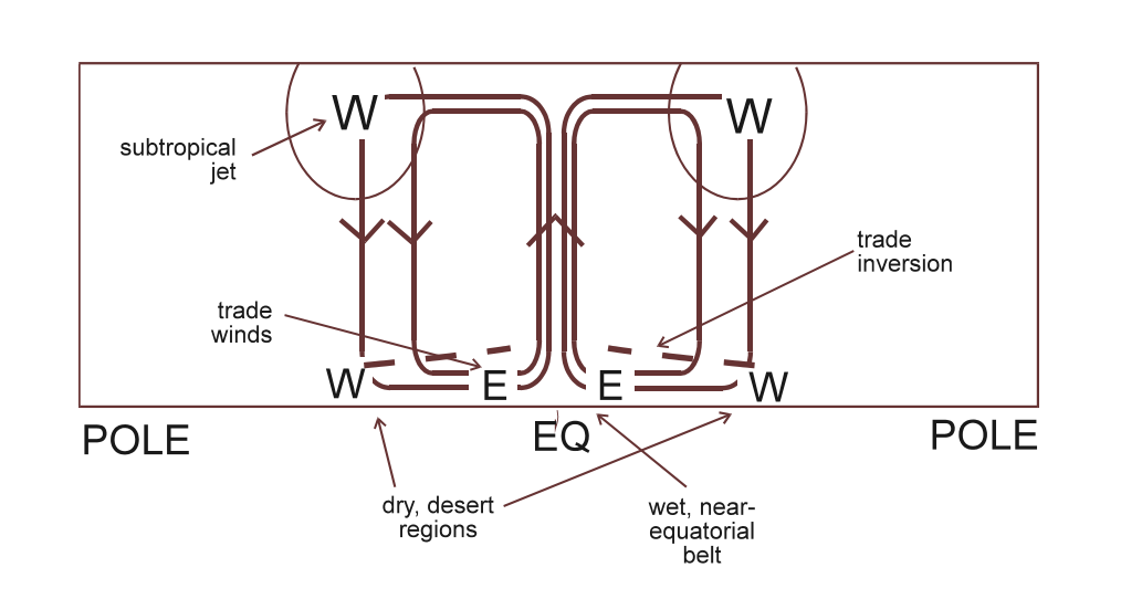
The Hadley cell is a region of convective overturning from about 0° to 30° N and S: the northern and southern extent shifts seasonally. Warm air rises at the equator, moves towards the poles, sinks in the subtropics, and returns along the surface towards the equator. Zonal winds are generated due to conservation of angular momentum. In the upper atmosphere, the westerly subtropical jet forms at the poleward boundary of the cell. Towards the equator, the easterly trade winds can be observed, although their speed is reduced by surface friction.
Poleward of 30° N and S, the Hadley cell breaks down. In a non-rotating Earth, the cell might extend all the way to the pole, but we observe that Coriolis deflection turns wind parallel to the equator at 30° where it sinks and returns to the equator. Temperature gradients poleward that cannot be equalized by convection lead to baroclinic instability.
Mid-latitude Eddies
Baroclinic instability leads to eddy formation. While there is a mid-latitude convective cell, its importance to heat transport is dwarfed by these eddies, which stir heat from the equator towards the pole. Eddy heat transport is horizontal, in contrast to the convective overturning at lower latitudes, and so varies less with height. The mid-latitude region dominated by weather systems extends from 30° to 60° N and S, where it gives way to the polar convective cell.
The seasonal variation and heat transport capacity of the Hadley and mid-latitude regimes can be demonstrated by examining data from the atmosphere.
General Circulation in the Atmosphere
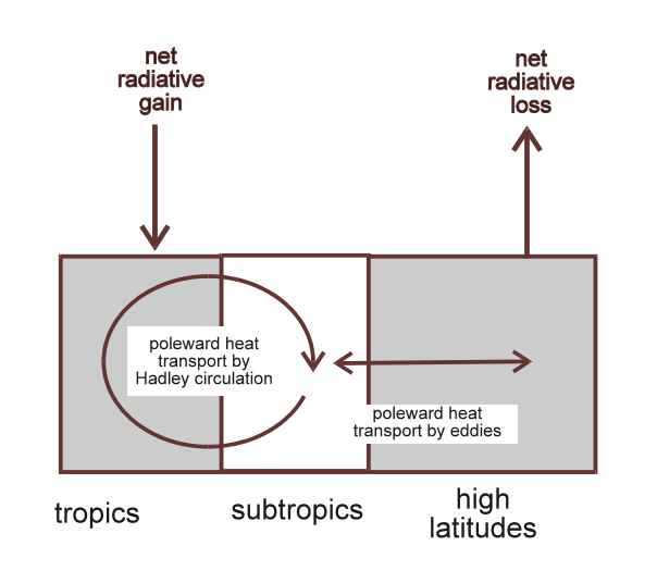
The earth receives heat energy from incoming solar radiation. Because the earth is round and its rotating axis is slightly tilted, the amount of income radiation is different depending on the latitude and time of the year. The mean incoming solar radiation is at a maximum in the tropics, and decreases as the latitude increases to the pole. The difference in radiative budget results in atmosphere’s meridional instability. To counteract the instability, the atmosphere transports heat from the equator poleward.
The meridional heat flux consists of two parts: the mean circulation and eddies. The mean circulation is most prominent in the tropics and called Hadley cell circulation, transporting heat from the equator to the sub-tropics. Eddies are the transient heat flux prominent in the mid-latitudes, transferring heat poleward. Together, they transport the heat from the equator to the pole.
Hadley Cell
We can plot climatological fields showing the meridional mean features of the atmosphere to observe the Hadley cell circulation. There are two phenomena that can be observed in the Hadley cell: the overturning circulation and thermal wind.
Overturning Circulation
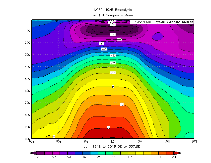
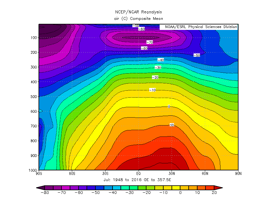
Figure 1. Zonally averaged temperature in January and July from 1948 to 2016. The warmest air is always at the tropics, but the temperature gradient is strongest over the mid-latitude in the northern hemisphere in January and in the southern hemisphere is July.
The overturning circulation functions by the convection of heat in the tropics. In Figure 1, the meridional temperature plot has its maximum in the tropics, where the incoming solar radiation is more perpendicular to the surface than the pole, hence the larger effective solar radiation.
In January when it is summer in the southern hemisphere, the solar radiation comes slightly more from the south, so the temperature peak is slightly to the south. As it is winter in the northern hemisphere, the temperature gradient in the northern hemisphere is larger than in the southern hemisphere. While in July where it is summer in the northern hemisphere and winter in the southern hemisphere, the temperature peak is slightly to the north, and the temperature gradient is larger in the northern hemisphere.
Because the incoming solar radiation in January and July is not equal in southern and northern hemisphere, the Hadley cell will not be two symmetrical cells over the equator. One cell will be weaker and one stronger, where it is easier to observe the stronger cell.
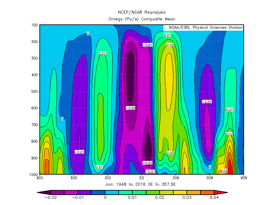
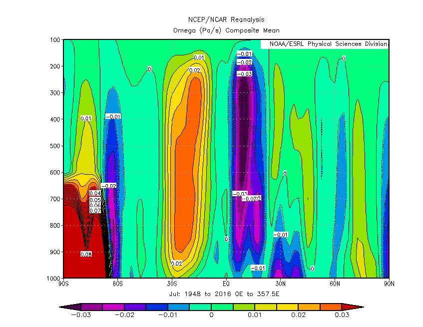
Figure 2. Zonally averaged vertical wind in January and July over 1948 to 2016. Positive direction is downward. The strongest upward flow is in the tropics, shifted to the south in January and to the north in July. The downward flow is strongest in the subtropics in the northern hemisphere in January and in the southern hemisphere in July.
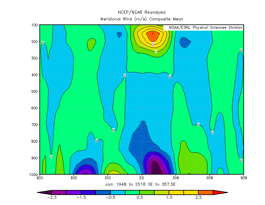
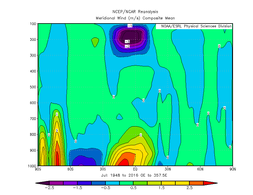
Figure 3. Zonally averaged meridional wind in January and July from 1948 to 2016. Positive direction is northward. In January, the strongest meridional winds are the wind in the northern tropics flowing toward North Pole in the upper layers and the wind flowing south toward the equator above the surface. In July, the strongest meridional winds are the wind in the southern tropics flowing toward South Pole in the upper layers and the wind flowing north toward the equator above the surface.
In January the temperature peak is in the southern tropics, so the strongest rising air is in the southern tropics (Fig 2). The air then moves northward following the largest temperature gradient into the northern hemisphere on the upper layers (Fig 3), then sinks down in the sub-tropics (Fig 2) and flow southward back to the equator near surface (Fig 3) to complete the circulation.
Similarly in July, the stronger Hadley cell has hot air rising from the northern tropics (Fig 2), moving southward following the stronger temperature gradient in the upper layers (Fig 3), sinking in the southern sub-tropics (Fig 2), and flowing back toward the equator near the surface (Fig 3).
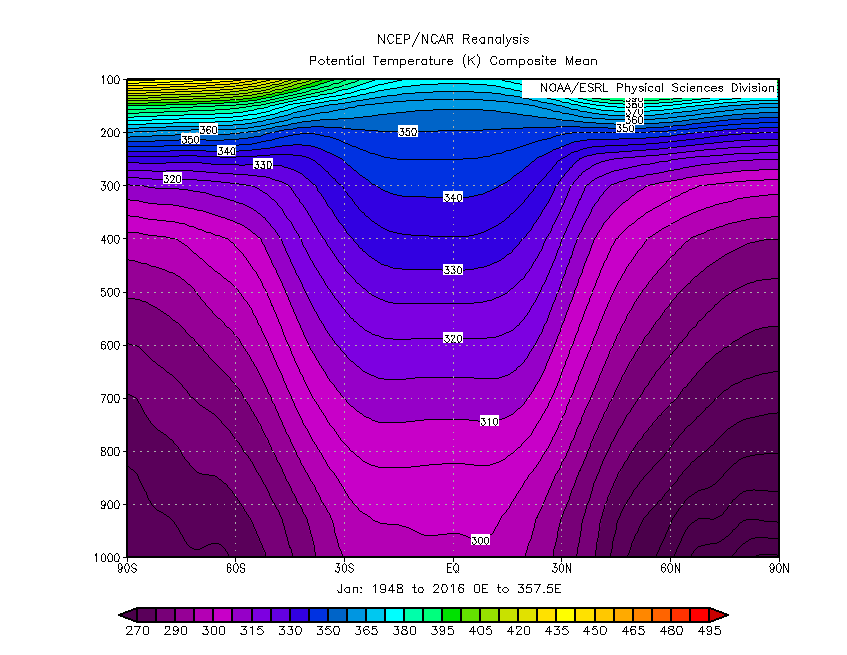
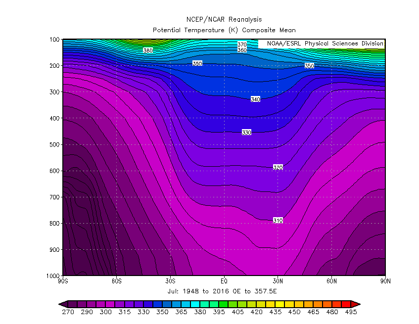
Figure 4. Zonally averaged potential temperature in January and July from 1948 to 2016. A dome of cold air is located over the pole. The temperature gradient is strongest over the mid-latitudes in the northern hemisphere in January and in the southern hemisphere is July.
Even thought the circulation consists of both the air flow poleward and equatorward, the amount of heat transport poleward is larger than the amount of heat transported toward the equator. From figure 4, the potential temperature in the tropics, where the Hadley cell circulation happens, has a rather flat gradient, showing that the Hadley cell is efficient in transporting heat.
Thermal Wind
From project 2, we know that thermal wind is strongest where the temperature gradient is largest. From Figure 1, the strongest temperature gradient is in the mid-latitudes of both hemispheres, and from figure 5 the strongest wind or jet stream is over the mid-latitudes.
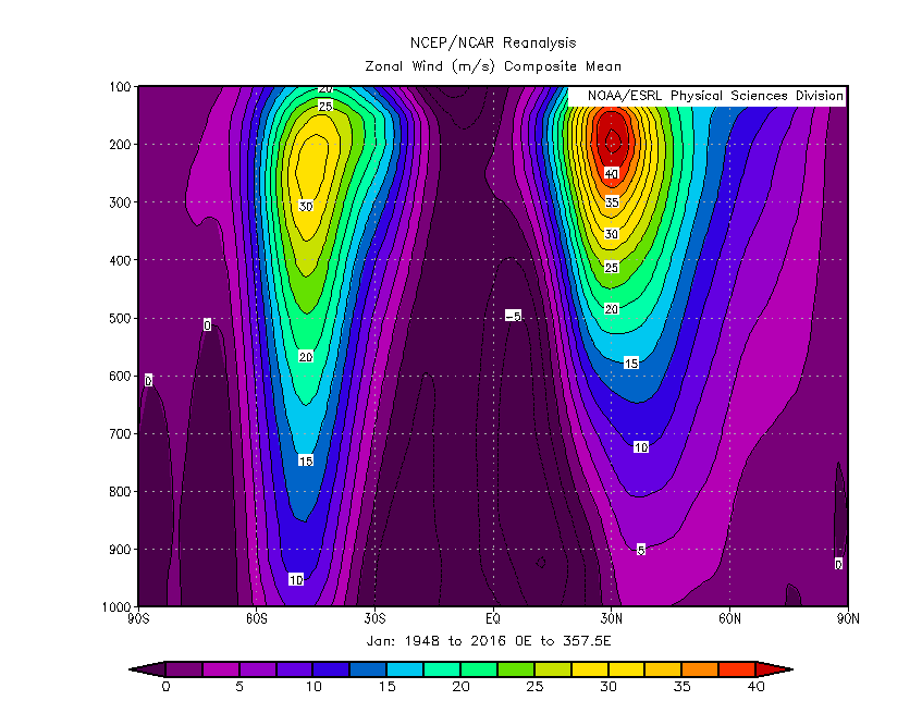
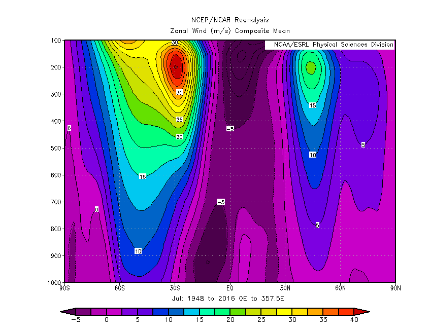
Figure 5. Zonally averaged zonal wind in January and July over 1948 to 2016. Positive direction is eastward. The strongest winds are eastward winds over the mid-latitudes in upper layers in both hemispheres, with the peak in the northern hemisphere in January and in southern hemisphere in July.
In the Hadley cell when air flows from the equator toward the pole, to conserve the angular momentum the wind speed increases. Moreover, the large temperature gradient in the mid-latitudes also marks the location where the heat flux from the Hadley cell stops, hence the temperature difference. The location and speed of the jet stream in the upper layers in the mid-latitudes also matches with the location and wind speed of a corner of Hadley cell where the air flow changes direction from poleward to downward.
Eddies
Transient eddies is the characteristic heat flux in the mid-latitudes. Even though mean circulation also occurs in this area (called the Ferrel cell), the transient eddy flux, which can be calculated by subtract the mean heat flux from the total heat flux, is more effective in transporting heat.
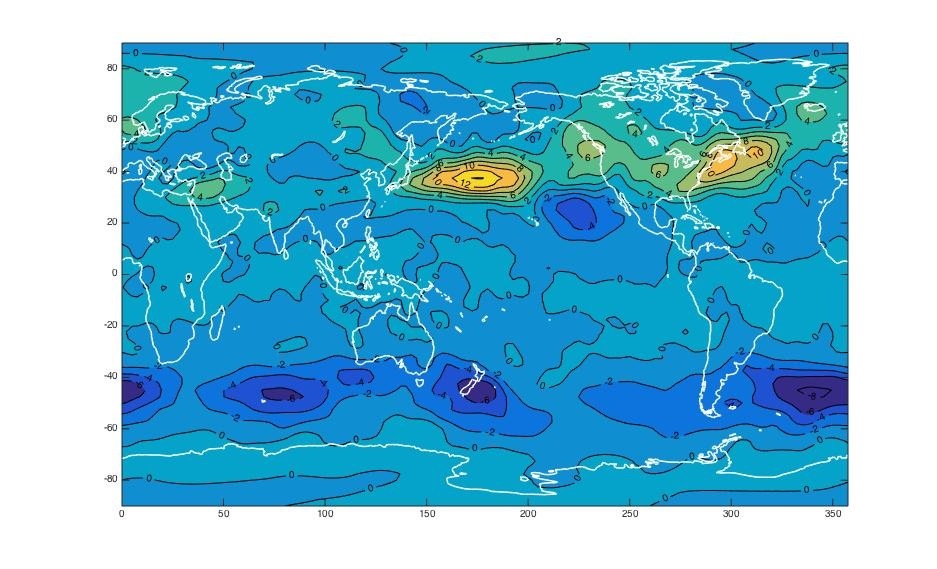
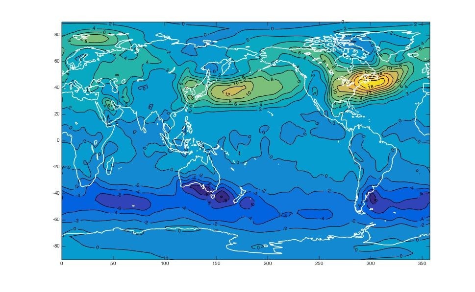
Figure 6. Transient heat flux at the level of 850 and 250 mbar respectively. Positive direction is going northward. Peaks exist in both levels of transient heat flux located in the mid-latitudes with flux going northward in the north hemisphere and going southward in the south hemisphere, but the magnitude of the peak flux is higher at the 250 mbar level.
From Figure 6, the transient heat flux has its peaks in the mid-latitude at both the 250 and 850 mbar levels. This contrasts with the heat transport in the Hadley cell circulation where the heat is transported poleward on the upper level and partially transported back toward the equator on the lower level. This characteristic also shows in figure 7 where the transient heat flux in the mid-latitude has the same direction in each hemisphere with the peak at 850 and 200 mbar levels.
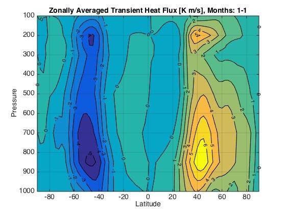
Figure 8. Zonally averaged transient heat flux is highest in the mid-latitudes with flux going northward in the north hemisphere and going southward in the south hemisphere at the 850 mbar and 200 mbar levels.
When the meridional transient heat flux is vertically integrated, the effectiveness of transient heat flux by eddies is shown by the clear peaks in the mid-latitudes, as shown in Figure 9. The eddies transport the heat to the north in the northern hemisphere, and to the south in the southern hemisphere.
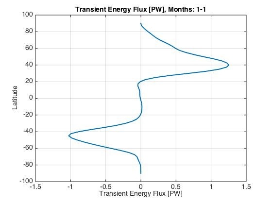
Figure 9. Anomaly of zonally and vertically integrated transient energy transport shows a peak in the mid-latitudes with flux going northward in the northern hemisphere and southward in the southern hemisphere.
When the heat fluxes from the Hadley cell circulation and transient eddies are combined, the heat is transferred effectively from the equator toward the pole in both southern and northern hemisphere. These two systems govern the climate pattern in their respective regions. In the tropics, the climate is largely due to the convective rising air into rainclouds. In the sub-tropics, the dry, warm sinking air creates dry deserts. In the mid-latitudes, the weather is influenced by fronts and hurricanes.
Tank Experiment
Two rotating tank experiments were set up. Tank rotation speed was the important parameter varied: one tank rotated at a speed of 1 rad s^{-1} and the other at 0.1 rad s^{-1}.
Slow Rotation Experiment
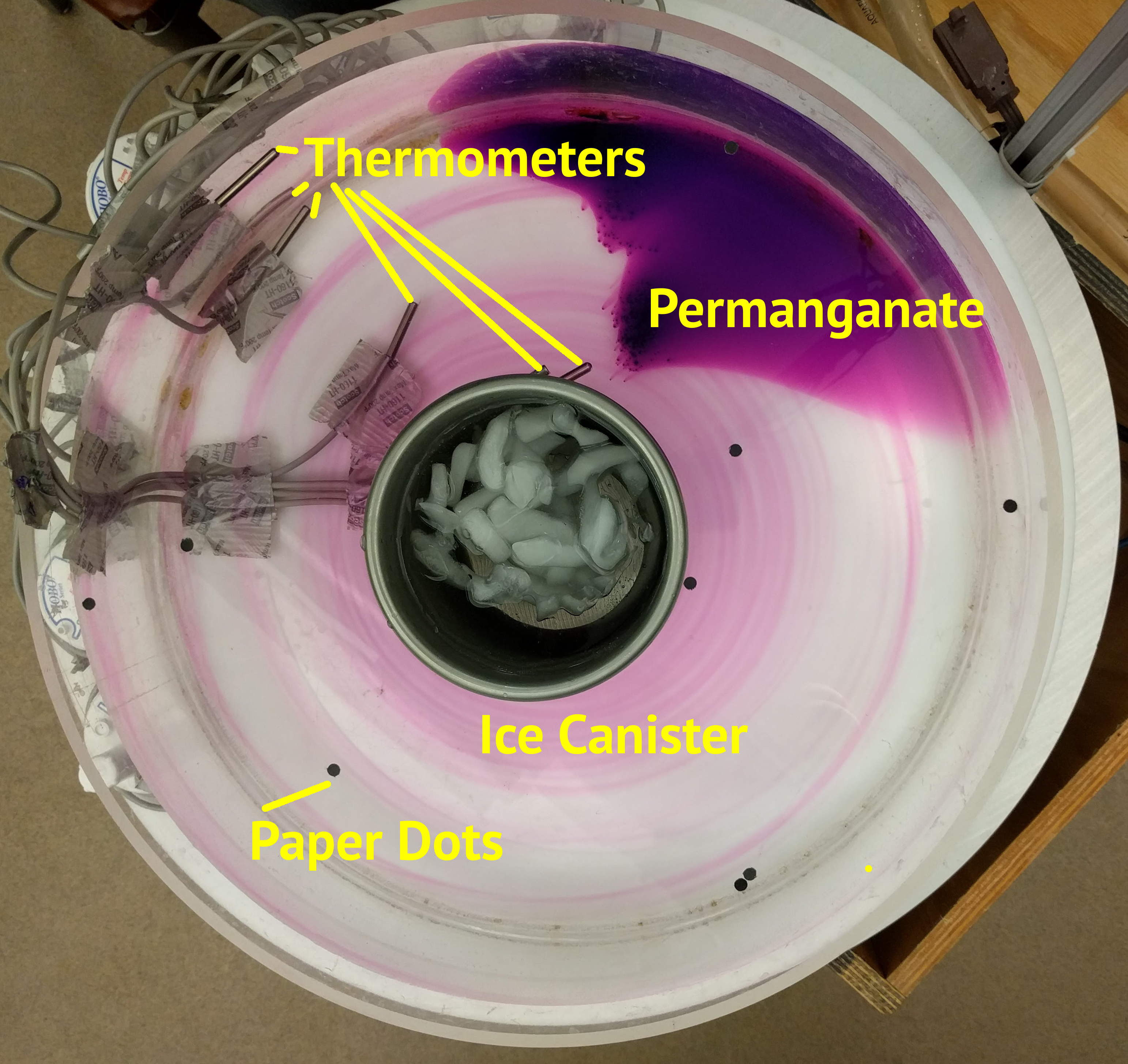
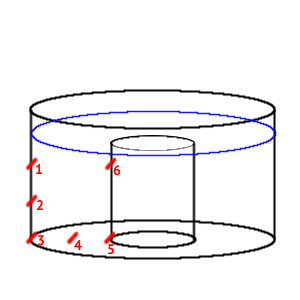
A metal canister of radius 12 cm was placed in the center of a tank of radius 22 cm. Six HOBO temperature sensors were taped to the tank in the arrangement shown in the figure below. The thermometer cables were taped along the bottom and edge of the tank to minimize interference with water flow. The tank was filled with still water to a height of 12.6 cm.
The rotating table was spun up to 0.1 rad s^{-1} and allowed to spin until a paper dot placed on the surface of the water appeared motionless to the overhead corotating camera, which was physically attached to the rotating table. The canister was filled with ice until full and then topped up with water.
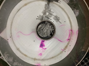
The surface speed of the water was measured by tracking black paper dots in the Particle Tracker application. The speed on the tank floor was measured by tracking the purple pigment trails from granules of potassium permanganate using timecoded screenshots in the Particle Tracker. Water speed shear between the top and bottom of the tank was measured with drops of blue food dye.
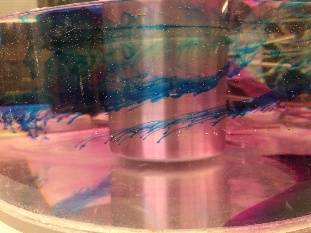
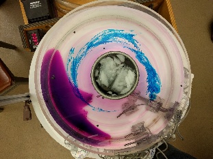
Fast Rotation Experiment
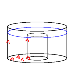
A metal canister of radius 18 cm was placed in the center of a tank of radius 31 cm. Again six HOBO temperature sensors were taped to the tank in the arrangement shown in the figure below. This arrangement differs from the first experiment: thermometers 1 through 5 were placed in a line radially from the tank center; thermometer 6 was placed between 3 and 4, on the bottom of the tank but 10 cm further in the clockwise direction. This arrangement was devised to capture thermal signatures of the eddies that were hypothesized to form. Thermometer 1 was placed at a height of 11 cm and thermometer 5 at a height of 9 cm. The tank was filled with still water to a height of 14 cm .
The rotating table was spun up to 1 rad s^{-1} and allowed to spin until a paper dot placed on the surface of the water appeared motionless to the overhead corotating camera. In this setup, the speed of the corotating camera was synced electronically with the table rotation speed through a computer interface. The canister was filled with 521.6 g of ice and then topped up with water.
Surface speed, bottom speed and shear were measured as in the previous experiment: paper dots, permanganate granules and food dye, respectively. Two colors of food dye were used to illustrate eddy formation: blue dropped in the colder water near the canister and red in the warmer water near the outside edge.
Results
Slow Rotation Experiment
Fast Rotation Experiment


Bibliography