Note: Casey wrote the section on the Hadley cell, and Kathryn wrote the section on the eddy regime.
Hadley Circulation
At the equator, solar radiation hits the Earth’s surface at a very steep (relatively direct) angle. At higher latitudes, solar radiation strikes the Earth at a shallower angle, and so the same amount of insolation is spread over a larger surface area. Thus, the planet is heated unevenly, and there is a net gain of energy at the equator and a net loss of energy at the poles. This uneven distribution of energy implies that there must be some heat transport from equator to pole.
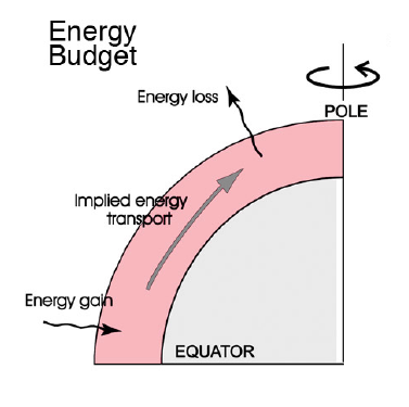
Modified from Marshall and Plumb, 2007.
In the tropical regions, where the Coriolis parameter is small (that is, where the effects of rotation are small), this heat transport is accomplished via the Hadley circulation.
The Hadley circulation takes place as follows: there is maximum solar heating at the equator, which stimulates rising motion. The flow then diverges aloft, moving poleward (which pole to which the air travels is dependent on which hemisphere is experiencing winter). As it moves poleward, the air becomes closer to the Earth’s axis of rotation. By conservation of angular momentum, the zonal velocity must increase. It reaches a maximum at the edge of the Hadley cell - about 30 degrees latitude, where the subtropical jet is located. From there, the air sinks back to the surface. As we will see, there is a horizontal temperature gradient in this region - thus, by the thermal wind relation, the zonal velocity of these air parcels must decrease as they sink back to the surface. Once at the surface, the air must move equatorward to close the cell. Because the parcels are moving further away from the Earth’s axis of rotation as they approach the equator, their velocity decreases zonally, eventually becoming easterly near the Equator. A schematic is presented below.
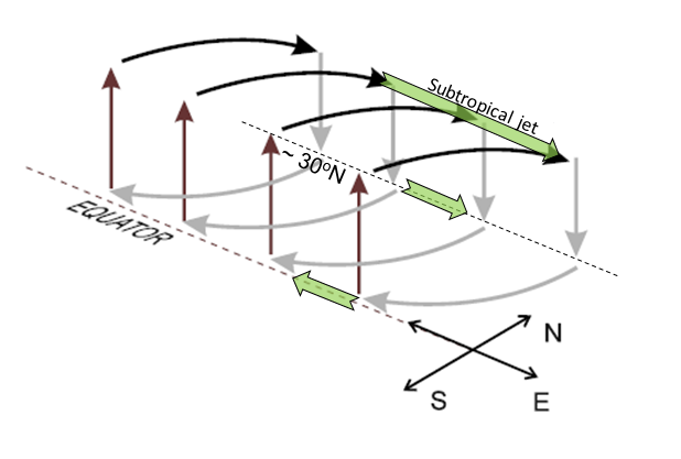
Modified from Marshall and Plumb, 2007.
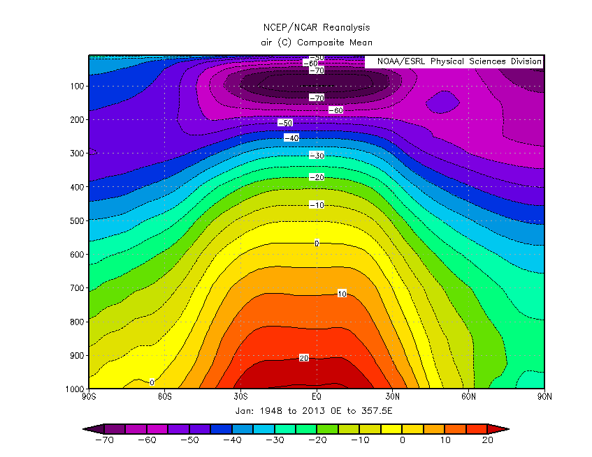
We can look for evidence of the Hadley cell by investigating climatological data for the months of January and July. All data and plots are from NCEP reanalysis data, available at http://www.esrl.noaa.gov/psd/cgi-bin/data/composites/printpage.pl.
First, let’s look at the zonally-averaged temperature structure for January and July:
JANUARY ZONAL MEAN TEMPERATURE (CELCIUS)
JULY ZONAL MEAN TEMPERATURE (CELCIUS)
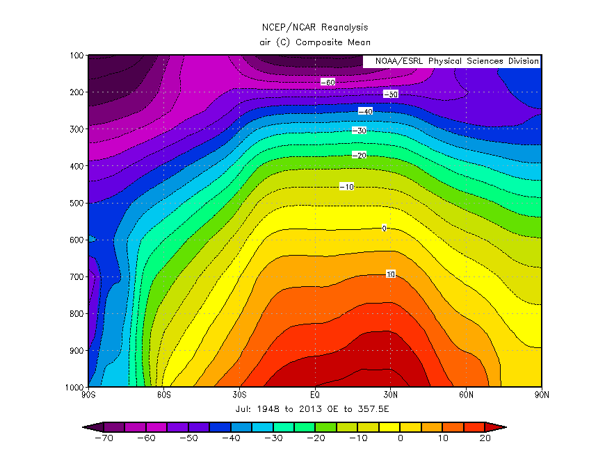
Notice that in both cases, the air temperature cools as we move from equator to pole. The thermal wind equation,
states that horizontal temperature gradients imply vertical shear in the horizontal wind. This relationship will be examined momentarily.
Before that, we can look at the zonal mean of potential temperature:
JANUARY ZONAL MEAN POTENTIAL TEMPERATURE (K)
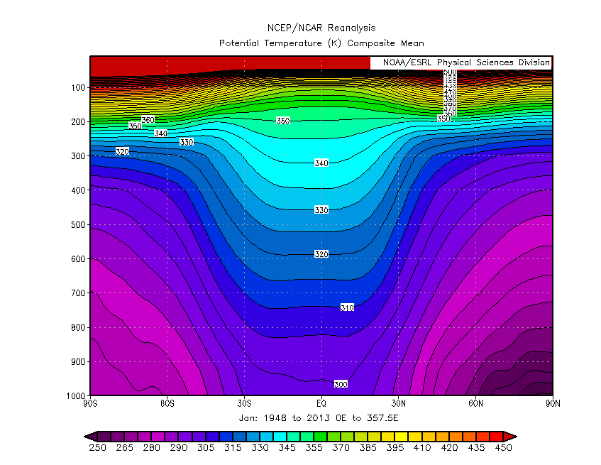
JULY ZONAL MEAN POTENTIAL TEMPERATURE (K) 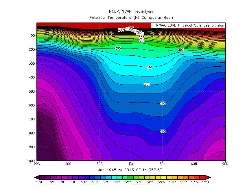
Once again, a sharp horizontal temperature gradient is evident at about 30-50 degrees latitude in both hemispheres in both January and July. Observe that above 200 mb, though, potential temperature is constant (or even slightly increasing). This will have implications for the thermal wind relation and the location of the jet stream. Finally, notice the domes of cold air situated over both poles. While these domes of cold polar air are present in both winter and summer, the dome of cold air is strongest in whichever hemisphere is experiencing winter.
Next, we can look at zonally-averaged zonal wind:
JANUARY ZONAL MEAN ZONAL WIND (m/s) 
JULY ZONAL MEAN ZONAL WIND (m/s) 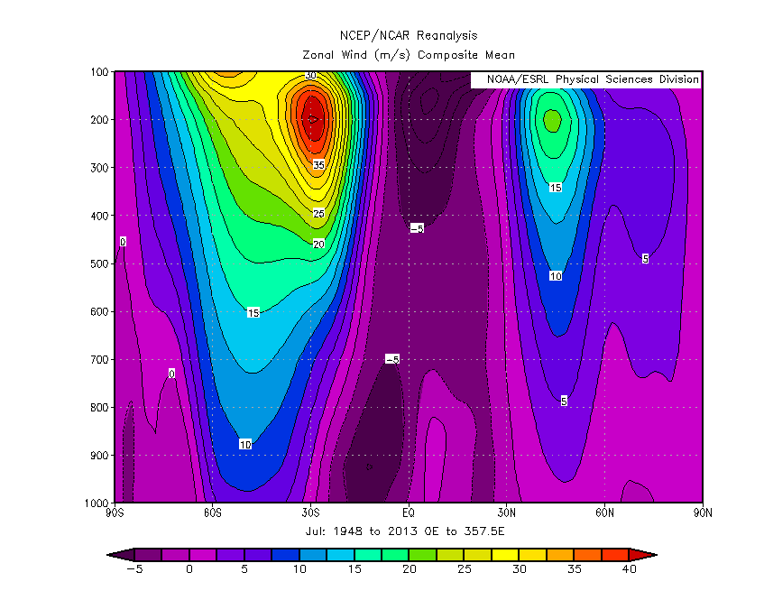
In both cases, the strongest wind speeds are located directly above the sharp temperature gradient observed in the plots of potential temperature---this is the location of the polar jet. The presence of these jets is consistent with the thermal wind equation: since the horizontal temperature gradient is strongest at about 30-40 degrees latitude, the strongest vertical shear of the horizontal wind should be present here. Notice also that although the jet is present over both hemispheres for all months, the jet is always strongest in the hemisphere that is currently experiencing winter.
We can be a bit more quantitative with our analysis and compare observed zonal wind speeds with those predicted by the thermal wind equation. All calculations are carried out at 30 degrees latitude and 500 mb. 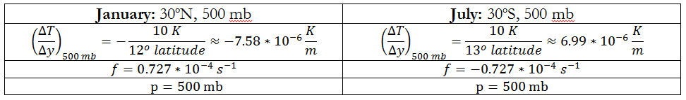
Therefore, plugging in the above values into the thermal wind equation and taking in the northern hemisphere and in the southern hemisphere,
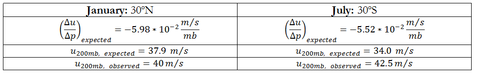
In both cases, the observed 200 mb wind speed is very close to the expected 200 mb wind speed (as predicted by the thermal wind equation). Thus, we can say that in both cases, the flow is in thermal wind balance.
Finally, it is not a coincidence that the jet is at a maximum at 200 mb. Below 200 mb, the polar front is quite strong. At and above 200 mb, however, potential temperature is almost constant with respect to latitude. Because there is very little horizontal temperature gradient, the zonal wind stops increasing with height, and a maximum wind speed is reached at 200 mb.
To move on, we can now look for evidence of the Hadley cell by observing the meridional structure of the wind.
First, we can look at vertical velocity, given in Pa/sec:
JANUARY ZONAL MEAN VERTICAL VELOCITY (Pa/sec) 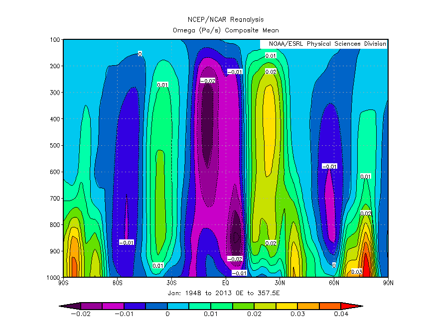
JULY ZONAL MEAN VERTICAL VELOCITY (Pa/sec)
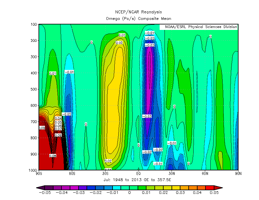
(Negative values correspond to upward motion, and positives values correspond to downward motion.)
In both cases, there is strong rising motion at the equator (again, this is caused by strong heating at the equator). In January, there is strong sinking motion at 30oN. There is also some sinking motion at 30oS, but since it is much weaker than the sinking motion at 30oN, we can say that the sinking at 30oN is a part of the Hadley cell, not the sinking at 30oS. By July, this strong sinking motion has migrated to 30oS.
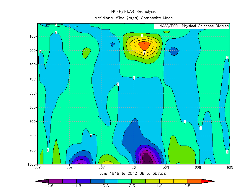
Next, we can look at the meridional wind to see if there is a north/south wind that connects these sinking and rising areas to form a cell:
JANUARY ZONAL MEAN MERIDIONAL WIND
JULY ZONAL MEAN MERIDIONAL WIND
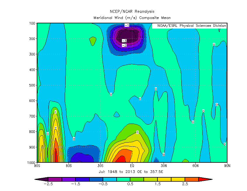
(Positive values are southerly flow, and negative values are northerly flow.)
Fortunately, in January, we see southerly flow aloft and northerly flow at the surface in the 0 to 30 degrees latitude region. This implies that the meridional flow connects with the rising and sinking motion to form a cell. The same thing happens in July in the southern hemisphere, but this time, the direction is reversed (northerly flow aloft and southerly flow at the surface).
It is helpful to plot these two fields simultaneously to get a better idea of the overall circulation:
ZONAL MEAN VERTICAL VELOCITY AND MERIDIONAL WIND
January on the left, July on the right. 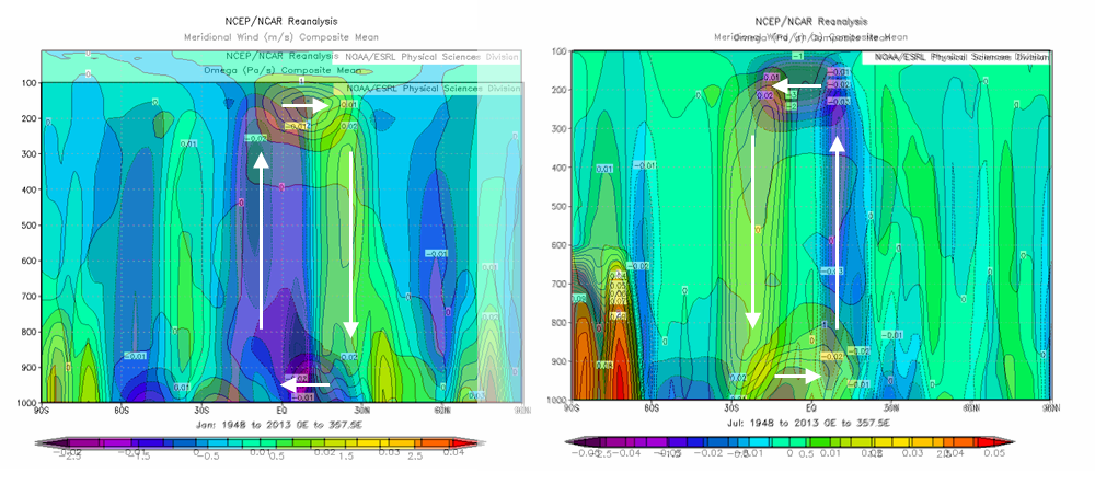
With this plot, it becomes clear that there is a cell in which air rises at the equator and then moves north or south toward whatever hemisphere is currently experiencing winter. At about 30 degrees latitude, the air once again sinks, and then moves equatorward, closing the cell.
Overall, this Hadley cell is the primary mechanism of heat transport in regions where the effects of rotation are small---the tropics. The Hadley cell transports energy by moving warm air poleward and cooler air equatorward. It is present in whichever hemisphere is experiencing winter.
- - -
To model the Hadley cell in the lab, we set up a circular rotating tank of water with a bucket of ice in the center. The bucket of ice is meant to represent the cold poles; the edge of the tank is relatively warmer and is meant to represent the equator. Thermometers were placed as such to get an idea of the structure of temperature inside the tank:
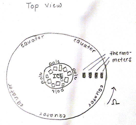
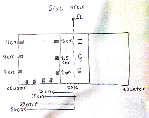
The tank was then rotated at 0.84 rpm. Black particles were placed on the top of the water to trace the surface currents. A co-rotating camera was placed above the tank to observe the flow in the rotating frame of references. Green dye was added to observe the flow within the fluid, and potassium permanganate crystals were dropped into the tank to observe the flow at the bottom of the tank.
Here are a few images of our experiment, with arrows drawn in to depict the flow:
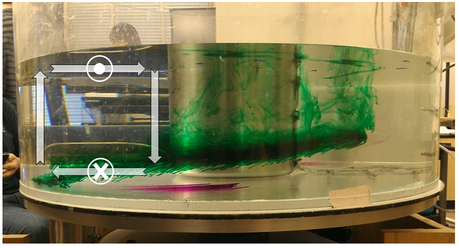
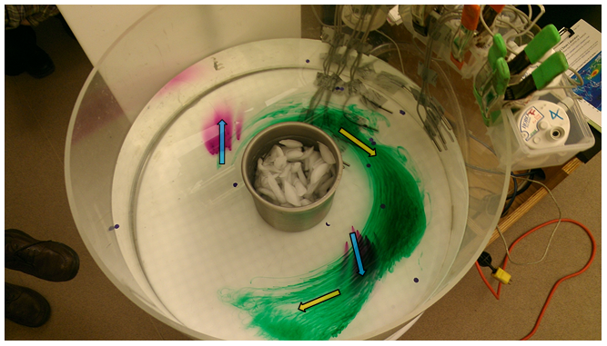
In the second photograph, the yellow arrows show the direction of surface flow and the blue arrows show the direction of the bottom currents.
The first photograph is a very good analogy between the tank experiment and the Hadley cells in the atmosphere. In the experiment, the center is cooled, and thus water in this region sinks (as in near the poles on the Earth). The water then moves toward the edge of the tank (“equatorward”). Near the edge of the tank, in order to conserve mass, the relatively warm water rises. At the surface, water flows inward, completing the cell (just as air in the atmosphere flows poleward aloft). Furthermore, there is a horizontal temperature gradient (as we will be shown soon), and thus the flow increases zonally with height. This vertical wind shear is evidence by the spiraling of green dye in the first photograph. This shear is also observed in the atmosphere, as shown in the previous section.
We were able to plot the tracks of the particles we placed on the surface of the fluid:
Particle Tracks for the Low-Rotation Tank Experiment
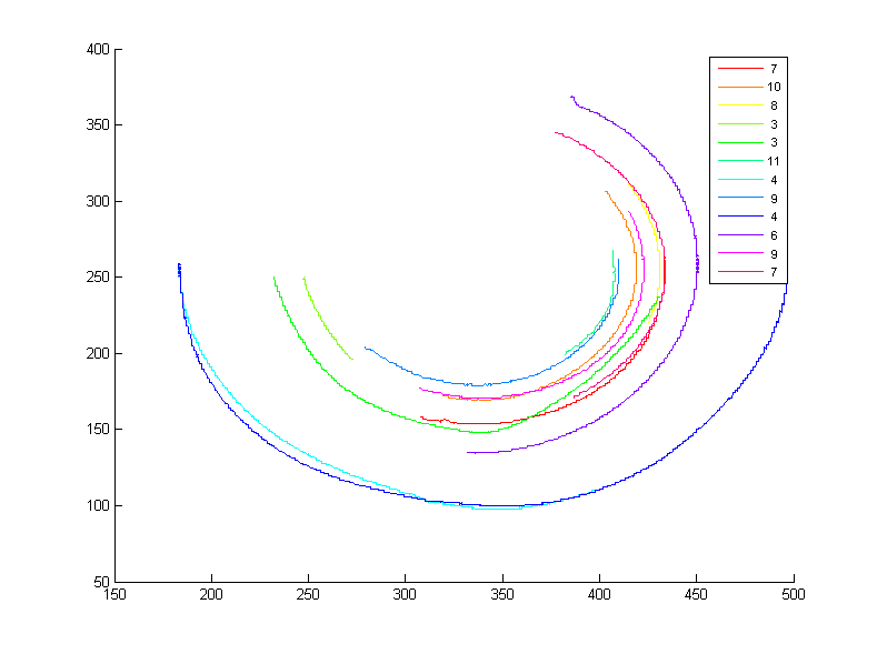
The numbers in the legend are the total speeds given mm/sec of the individual particles. These particles spiral cyclonically around the ice, just as air circles the poles cyclonically in the atmosphere. Furthermore, the particles closest to the center travel the fastest, because this is the region in which the temperature gradient is strongest. This is analogous to the jet over the polar front in the atmosphere.
Next, we plotted the temperature from the sensors on the bottom of the tank:
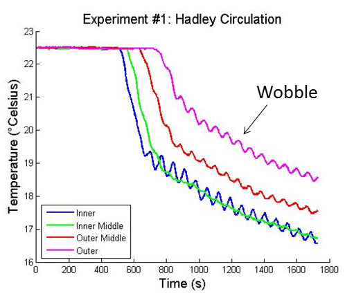
From the plot, it is evident that we placed ice in the center at about t = 600 seconds. Notice that the circulation doesn’t happen throughout the entire tank right away; instead the cold water propagates outward along the bottom of the tank relatively slowly, taking about 150-200 seconds to reach the outermost sensor.
Another interesting observation is that there is a “wobble” in the data. These wobbles have a period exactly equal to the rotation rate of the tank; we think the bottom of our tank was not level, and so the water “sloshed” around as the tank rotated, causing strongly periodic oscillations in temperature.
We were also able to plot the temperatures recorded by the sensors along the side of the tank:
By comparing middle to middle, outer to outer, etc., it is clear that the horizontal temperature gradient is not constant with height; instead, the temperature gradient decreases as we move upward in the tank. Using the above measurements, we obtained an average horizontal temperature gradient of 8.23 K/m.
We then sought to apply the thermal wind equation for water:
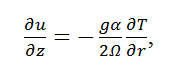
where dT/dr = 8.23 K/m, α (the coefficient of thermal expansion) is 207 * 10^-6^ K^-1, and Ω = 0.088 rad/sec. These values gave us a du/dz of 9.5 * 10^-2 m/s/m.
Making the assumption that the flow at the bottom of the tank was close to zero, this gave us an expected surface velocity of 1.42 cm/sec. Unfortunately, this is significantly larger than the observed surface velocities of 0.5-1 cm/sec. We think that the source of this error is that our value for dT/dr is a rough estimate; dT/dr is actually varies with height, so using a single value for the horizontal temperature gradient (instead of integrating vertically) is likely to introduce some error. Nonetheless, we think these values are close enough to be believable.
Altogether, the low rotation experiment was a great analog to the atmosphere. In both cases, air rises in relatively warm areas and sinks in relatively cool areas. Meridional flow completes the cell. Overall, these cells are responsible for transporting energy poleward in low-rotation regimes.
Eddy Circulation
Compared to low latitudes which we discussed above, the middle latitudes of the earth have a slightly higher Coriolis parameter, and thus experience more effects from the earth’s rotation. The uneven heating of the earth tells us that heat must still be transferred from the equator to the pole across the mid-latitudes, but because of the higher rotation rate, the mechanism of heat transfer is quite different. In mid-latitudes, the Hadley cell described above breaks down. An argument of angular momentum conservation explains the break-down.
In the Hadley cell, parcels of air move poleward conserving the angular momentum they had at the equator. Angular momentum has components from both the rotation of the earth and the zonal velocity of the parcel within the earth’s rotating frame (Equation 1). 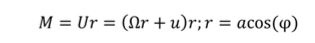
Equation 1: Angular momentum contributions from the earth's rotation and u, the zonal velocity of the parcel.
Since the parcels of air move to a smaller radius when they move poleward, their zonal velocity must increase in order for the total angular momentum to remain the same. The functional form of this increase is derived below (Equations 2-4).
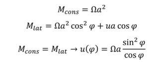
Equations 2-4: Derivation of the zonal velocity at various latitudes due to angular momentum conservation alone. Note that the resulting equation gives an infinite velocity at the poles.
If parcels of air were to rise from the equator with zero zonal velocity and move poleward conserving their total angular momentum, the equations above tell us that the zonal velocity at the pole would be infinite. This is clearly unphysical. Therefore, there is a point at which the Hadley cell must break down, and heat must be transported some other way.
The Hadley cells are observed to break down at about 30 degrees North and South; instead, eddies in the atmosphere transport heat above at those latitudes. Eddies can be seen in the satellite image below, carrying large bands of swirling clouds across the central United States.
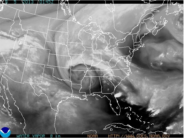
Source: NOAA GOES-E satellite; http://www.goes-arch.noaa.gov/cgi-bin/post-archive. Data from May 5, 2013.
Eddies can also be seen in the oscillating fronts which separate the cold air over the pole from the warm air in mid-latitudes. In the colorful picture below, from January 2013, there are six or seven oscillations of this surface over the pole.
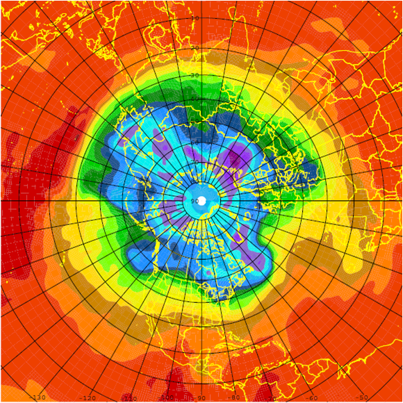
Layout of potential temperature curves over the North Pole at the 500 millibar surface. Cold temperatures are purple and blue; warm temperatures are red and orange.
These eddies are efficient at transferring heat in the atmosphere. Through temperature fluctuations (T’) and velocity fluctuations (v’), they carry large amounts of heat from the equator to the poles. A plot of zonally averaged head flux from the north pole to the south pole shows maximum heat transfer at approximately 40 degrees North and 40 degrees South, where the eddies are transporting heat. It is also interesting to note that the heat flux is greatest in the 700-1000 millibar range, where weather systems occur in the atmosphere. This suggests that weather systems are also a mechanism for heat transfer.
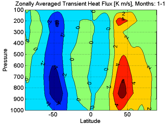
Heat flux over height and latitude. The largest heat flux is in the lower portions of the atmosphere at 40N and 40S.
If one vertically integrates the heat flux, the heat flux as a function of latitude shows the action of eddies even more clearly. The maximum eddy transport is directed northward at 40 degrees North and southward at 40 degrees South.
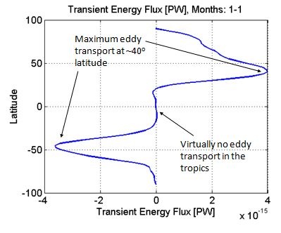
Vertically-averaged heat flux as a function of latitude. Data taken during January.
Once we understood the role of the eddies in the atmosphere, our goal in this project was to recreate these eddies using the tank experiments developed above. Using the same set-up as the Hadley cell experiment, we simply changed the rotation rate to be considerably higher. The experiment used:
- Rotation rate = 7 RPM
- Bucket holding 1.2 kgs of ice
- Temperature sensors and paper dots for measurements
- Red and green dye added
Tank Experiment for the eddy circulation:

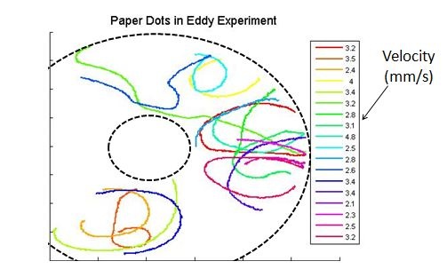
We observed the eddies in the tank by tracking the motion of paper dots along the surface of the tank. Each dot was given a different color, leading to a very colorful illustration of the swirling eddies in the tank:
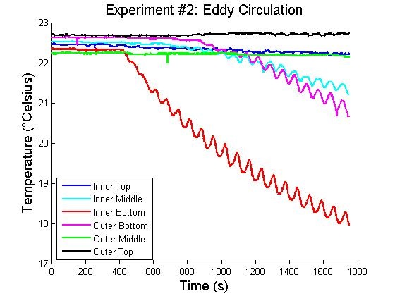
Next, we measured temperature fluctuations within the eddies using thermisters placed on the bottom of the tank. As plumes of warm and cold water flowed over the thermisters, the sensors recorded the temperature variations. The temperature variations are shown below.
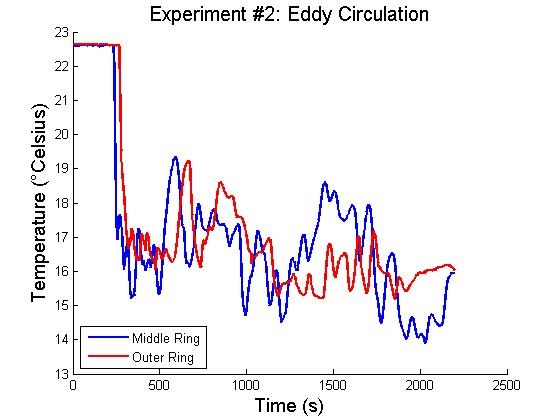
Temperature fluctuations measured at the bottom of the tank during the Eddy Circulation experiment.
Then, we computed the heat transported by the eddies and compared it to the heat absorbed by the melting ice. We expected a match within an order of magnitude; we did not expect a closer match because we only had a few temperature sensors and we were only able to see a tiny piece of what the eddies were doing throughout the tank.
We estimated the fluctuations in temperature and velocity by using the standard deviation of our measurements. The standard deviation of the temperature measurements was approximately 1 degree Celsius, and the standard deviation of the velocity (radial component only) was approximately 0.7 mm/s.
We calculated the flow of heat into the ice and the flow of heat transported by the eddies. The power required to melt the ice is the latent heat of the ice times the amount of ice, divided by the amount of time it took for the ice to melt (35 minutes in this experiment). The heat transported by the eddies is the mean temperature fluctuation times the velocity fluctuation (both given by standard deviations of the data), then vertically and horizontally integrated over a "control cylinder" of an average radius of 0.19m. This radius is located between the inside and outside temperature sensors (Equation 5).
Using these formulas, we found a rough agreement between the eddy transport and the power required to melt the ice. The order of magnitude was the same, even if the numbers were different. The comparison was:

The agreement in our data was not perfect, but it matched within an order of magnitude. The causes of the discrepancy may include the fact that our only temperature measurements in the center of the tank were taken at the bottom of the tank; the behavior of the eddies may not have been uniform in the vertical direction, but we could only measure at the bottom. Our measurements on the edges of the tank were still not able to constrain exactly what was happening in the water column at our chosen "control cylinder".
Our tank experiment was successfully able to model some of the characteristics of eddy transport in the atmosphere. It was able to redistribute heat to melt the ice and create turbulent swirling patterns on the surface, much like the atmosphere at mid-latitudes. The qualitative connection between the two systems is clear in the image below.
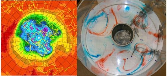
Qualitative comparison between atmospheric system and the tank experiment.
Eddies, like the Hadley circulation, are an important mechanism for heat transport in the atmosphere. Eddies in part determine the weather patterns around mid-latitude cities like Boston. They also allow the polar regions of the earth to receive some of the solar energy which is incident on the earth's surface at the equator. In other words, they keep the poles warmer than they would be otherwise. The transport of heat due to eddies has profound impacts on the climate of the mid-latitudes and polar regions of the earth, which in turn has important consequences for the habitats in which we can live.
Through this project, we were able to build our understanding of eddy transport in the atmosphere and replicate its action in the lab. If we were to repeat the experiment, it might be interesting to do a concurrent experiment to melt the same amount of ice in an identical but non-rotating tank of water. It would allow us to see how effective the eddies are at transporting heat compared with the simpler process of convection in a non-rotating system. I would predict that the ice melts much faster in the rotating system because the turbulent eddies shuttle cold water away from the ice cubes more effectively than simple convection. It would be fun to perform the comparison.