Chris and Violet worked together on this project. Chris focused on the eddies section and Violet focused on the Hadley cell section.
------------------------------------------------------------------------------------------------------------------------------------------------------------------------------
Hadley Cell
by Violet Luo
What would happen if the Earth stopped rotating? 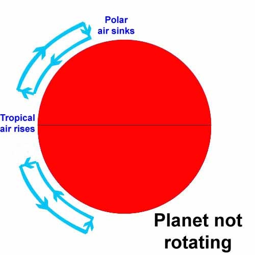
The picture is available at: http://www.met.reading.ac.uk/~sgs02rpa/CONTED/cl-intro_files/no_rot_earth2.jpg
In a non-rotating environment, there is only one circulation in each hemisphere. Air moves to balance the uneven distribution of energy on the Earth. In the equatorial areas which receive more solar energy, the warmer air rises, flows poleward above the surface, and sinks near the Pole where receives less solar radiation; then the colder polar air flows equatorward near the surface, forming a simple cycle of air movement.
Why is the assumption impossible?
U= Ωr+u,
where the angular velocity of the earth Ω=7.29 ×10^5 rad/s, the horizontal component of the earth’s radius vector r=acosφ, U is the relative zonal wind velocity to the earth, and u is the zonal wind velocity on the Earth.
M=Ur,
where M is the angular momentum. When plug MO= Ωa^2 in,
u= Ω(a2-r2)r.
At the Pole where r=0, the zonal wind velocity is infinite, while in fact the average polar wind velocity must be finite. Therefore, the simplification that the Earth is non-rotating is incorrect.
Tri-Cellular Circulation 
The picture is available at: http://coolgeography.co.uk/A-level/AQA/Year%2013/Weather%20and%20climate/Structure/Tri-cellular%20Model.htm
Regarding the rotation of the Earth, the simple cycle grows more complicatedly to the tri-cellular circulation, which truly describes how the air moves on the Earth. In the three cells, the Hadley Cell near the equator and the eddies will be fully discussed.
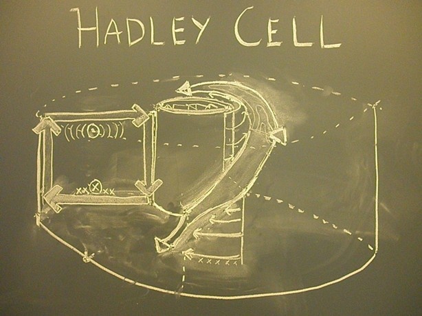
Hadley Cell
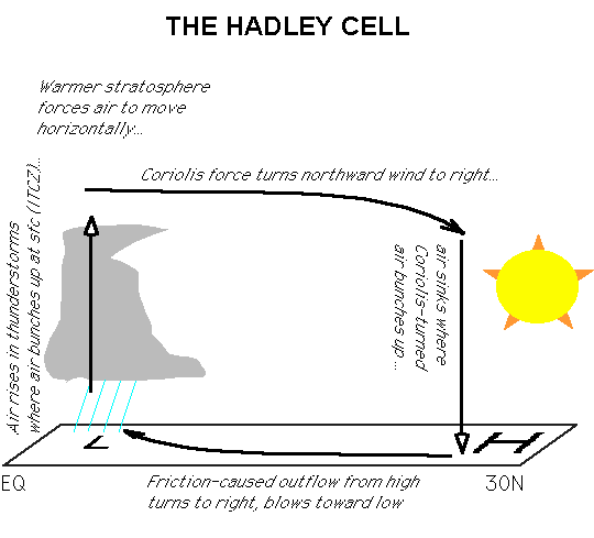
The picture is available at: http://sparce.evac.ou.edu/q_and_a/air_circulation.htm
1735, George Hadley proposed a general circulation which is exactly as Figure 1. It was proved later that due to the angular momentum constraints, the warmer equatorial air rises, poleward flows 15-20 km above the surface, sinks in the subtropics, and flow equtorward near the surface. Because of the Coriolis force, the currents near the surface turn to right and form north-east trades in the northern hemisphere and south-east trades in the southern hemisphere.
To fully investigate the Hadley Cell, atmospheric data are retrieved from: http://www.esrl.noaa.gov/psd/cgi-bin/data/composites/printpage.pl
Potential Temperature
January
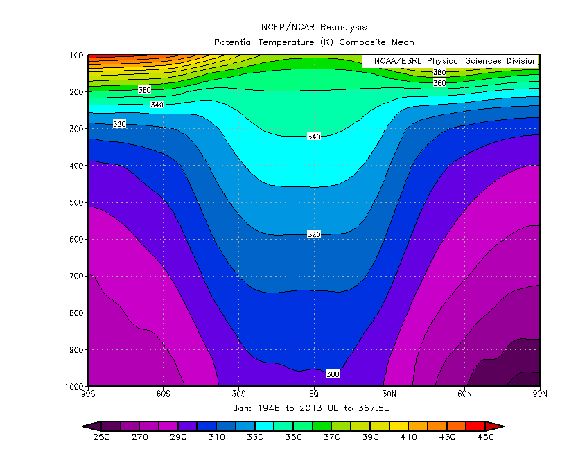
July
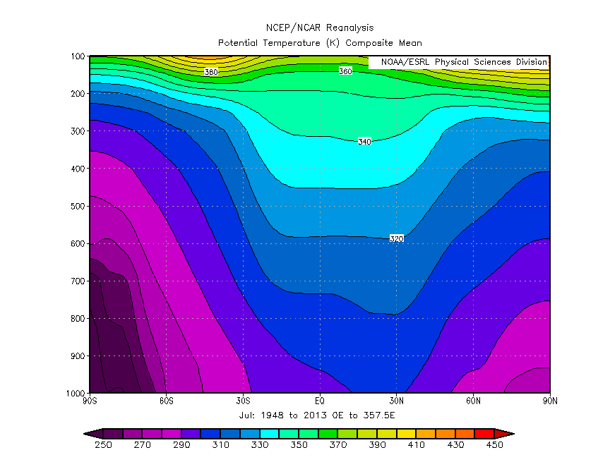
Above are two potential temperature graphs in January and July, which show the zonal mean potential temperature distribution from 1000mb to 100mb because data are unavailable below 100mb. The strongest gradients occur in the middle latitudes and shift a little toward the summer hemisphere. There is no large heat difference in tropical regions because of the Hadley circulation.
Zonal Wind
January
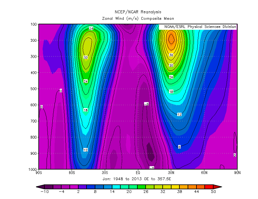
July
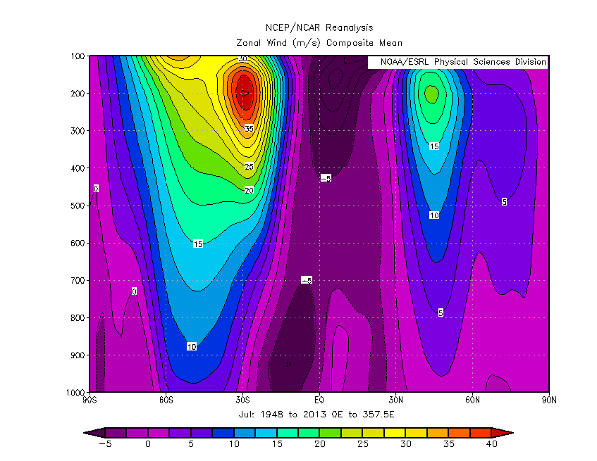
In the upper part of the Hadley circulation, as air moves away from the equator, the Coriolis parameter becomes much larger and turns the wind to right, resulting in an easterly zonal wind component to the flow in the northern hemisphere. In addition, zonal wind is stronger in the winter hemisphere.
Meridional Wind
January
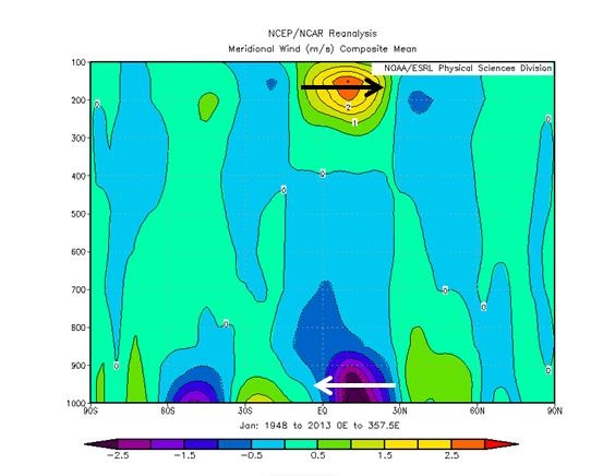
July
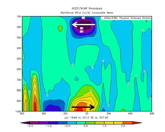
Air is descending towards the surface at 30N in January, but it cannot build up at the ground, so there is a northerly wind, which is known as negative meridional wind, between 0N and 30N in January. The same is true for the southerly wind around a height of 100 mb; between the flow up at 0N and the flow down at 30N, positive meridional wind must move towards the north in order for the circulation to be completed. The same pattern occurs in July, but it is much stronger in the southern hemisphere because the whole Hadley cell is stronger in winter hemisphere.
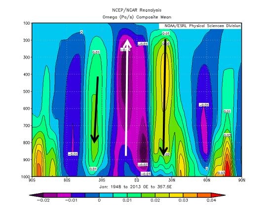
Omega
January
July
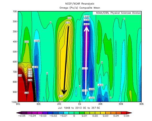
In January, the equatorial air rises and descends towards 30N and 30S. Because eddies are stronger in winter, the main Hadley circle occurs in the northern hemisphere between 0 and 30N. The same pattern is stronger in the southern hemisphere in July.
Transient Heat Influx
Transient Heat Influx in January
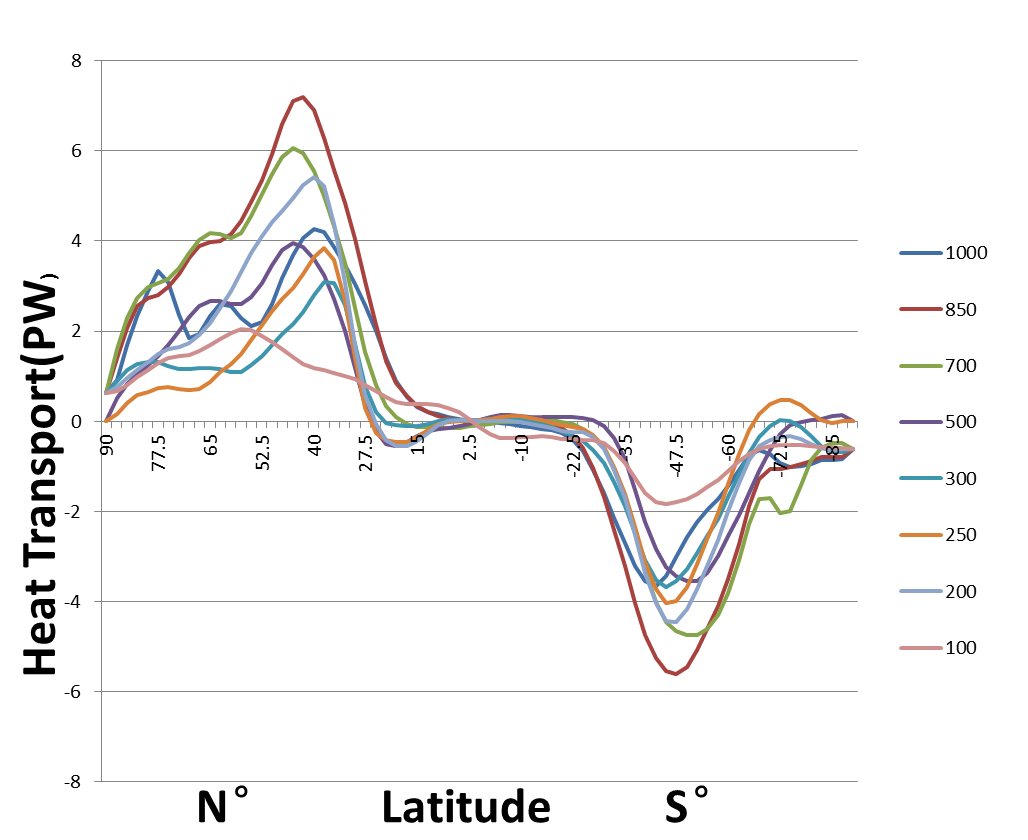
Transient Heat Influx in July 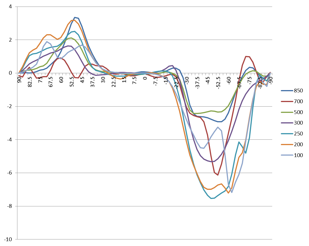
Because eddies are stronger in winter, the magnitude of transient heat influx is larger in winter hemisphere. The flat line between approximately 30N and 30S indicates that the Hadley circulation is efficient in transporting heat between these latitudes, so there is no large heat difference. It can also be concluded that the temperature is warmer in the middle latitudes than if there were no circulation.
Conclusion
Hadley Cell is a circulation transporting heat in the tropics. It carries the warmer air near the equator to 15-20km above the surface and descends at latitude 30. It is stronger in the hemisphere which is experiencing winter.
Laboratory Analogue
by Chris Klingshirn
This section describes the design of a laboratory experiment to simulate the large-scale general circulation of earth's atmosphere and compares the results of the experiment to the predicted behavior.
This section describes the design of a laboratory experiment to simulate the large-scale general circulation of earth's atmosphere and compares the results of the experiment to the predicted behavior.
Background
It is observed that the mean differences in near-surface temperature and outgoing radiation between the earth's equatorial and polar regions are significantly smaller than the difference in incident solar radiation between the tropics and the poles. This observation implies the existence of a net equator-to-pole transport of energy [1]. One of the mechanisms responsible for this energy transport is the atmospheric general circulation, a net poleward transport of warm tropical air into colder polar regions.
Experimental Design
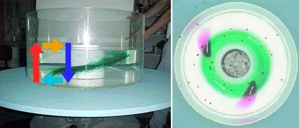
We attempted to duplicate the mechanism and the effects of the general circulation by constructing a physical analogue in the laboratory. The dominating feature of the general circulation is a radial temperature gradient in a rotating frame of reference. In the experiment, a rotating tank of warm water simulated air on the rotating earth, and a centrally positioned metal bucket containing ice and cold water simulated the cold pole:
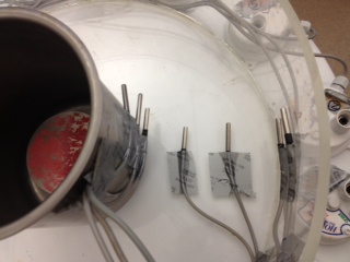
The apparatus consisted of a rotating cylindrical tank of warm water, representing warm equatorial air, with a cold metal bucket of ice-water at the center to represent the cold polar air.
Thermometers were placed in the tank at two radii and at several heights on the inner and outer walls:
Results
Hadley Circulation Regime (1 rpm)
The tank was set rotating at a relatively slow 1 rpm, for a Coriolis parameter f=0.21, to simulate the dynamics of Hadley circulation in the earth's equatorial regions where f is small compared to higher latitudes (on a sphere, f=2Ωsinφ, where φ is latitude).
We observed an inward surface flow, which had positive tangential velocity, and outward near-bottom flow with negative tangential velocity:
Adapted from http://paoc.mit.edu/labguide/circ_exp_slow.html
Measurements showed a radial temperature gradient that was approximately constant in time:
Expected Behavior
The radial temperature gradient causes radially-asymmetric convection, with water near the cold center cooling, becoming more dense and sinking. This flow leads to radial motion towards the center at the surface and away from the center at the bottom of the tank. This radial flow is distorted tangentially as a consequence of the conservation of angular momentum, which is proportional to the square of the distance to the center of rotation; as a particle near the edge moves inwards, it acquires a positive tangential component to enforce angular momentum conservation, or similarly, a negative tangential component if the particle is moving radially outwards:
_From http://paoc.mit.edu/labguide/circ_exp_slow.html._
The closeness of the analogue behavior to the predicted behavior can be determined quantitatively via the thermal wind relation:
Using dT/dr=3.3 C/m at the surface and known constants, one may compute compute du/dz=0.0314 cm/s/cm. Given a depth of 12 cm and assuming that the velocity at the bottom is negligible, this gradient implies u=0.38 cm/s at the surface, which is close to the 0.46 cm/s measured by tracking a paper dot placed on the surface with a camera mounted in the rotating frame.
Unstable Eddy Regime (5 rpm)
After the simulation of Hadley circulation, the experiment was conducted again with a tank rotation rate of 5 rpm to simulate the general circulation at higher latitudes on the earth.
The flow became unstable and was no longer radially symmetric, but consisted of several eddies:
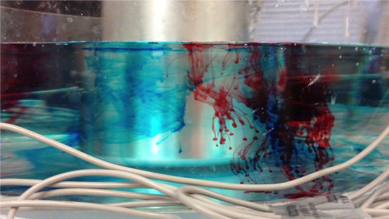
These eddies are analogous to cyclonic weather systems seen in earth's mid-latitudes.
The thermometers were re-configured and one more was added, for a total of eight. Three were arranged on the bottom at 4-cm intervals on the radial arc for r=8 cm:
Unlike the predictable temperature profiles of the 1 rpm trial, the temperature profiles in the 5 rpm case are pseudo-periodic with amplitude ~0.5 C and exhibit large fluctuations:
The oscillatory nature of the temperature curves is the result of eddies, each with a warmer and a cooler component, repeatedly passing over the thermometers.
Energy Flux Toward the Cold Pole
One can compute the efficiency of the eddy-induced heat transport by comparing the mean thermal power required to melt the ice in the bucket with an integrated thermal power flux computed from measurements of velocity and temperature anomalies in the tank.
Given a mass of ice of 0.992 kg which melted in 1740 s, and the latent heat of ice, one finds that a mean power of 190 W contributed to melting the ice.
The mean power flux carried by eddies across a specific radius within the tank may also be computed. Integrated in the vertical and around the tank,
where v'T' represents the product of temperature and velocity anomalies. Using a mean surface velocity of 0.218 cm/s at a radius of 0.106 m and assuming a linear velocity increase in height from the bottom, an estimated mean temperature anomaly of 0.5 C, and a depth of 0.1 m, one obtains a mean power of 152 W being transported towards the bucket of ice by eddies. This value is plausible because it is slightly lower than the 190 W power required to melt the ice, with the difference likely being accounted for by thermal power from the warm air in the laboratory. It is clear that the eddy heat flux is quite efficient at transporting heat from the edge of a rotating system towards the center.
Conclusion
The tank analogue successfully modeled both the Hadley circulation and eddy circulation regimes of the atmospheric general circulation. We were able to simulate the latitude dependence of the earth's Coriolis parameter by adjusting the rotation rate of the tank, with a higher rate to simulate the greater Coriolis parameter at higher latitudes. The Hadley simulation reproduced both the meridional and zonal structure of the Hadley circulation on earth, and the eddy simulation reproduced the instability of cyclonic weather systems.
References
[1]. http://paoc.mit.edu/labweb/notes/chap5.pdf
1 Comment
MIT Student