Because of the orientation of the Earth with respect to the Sun, there is significantly more solar heat flux at the Equator than at the poles. There exists a temperature gradient between the Equator and the poles; however, the gradient would be much larger if there were no meridional heat transport. In order to reach the temperature gradient observed today, there needs to be a pole-ward flux of about 6 petawatts, which includes both atmospheric and oceanic heat transport (Marshal & Plumb 2008).

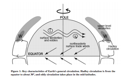
Figure 1 reveals the general circulation of the atmosphere. Near the equator there is uprising of hot air that moves to the low-pressure poles. The majority of this air sets at approximately 30°. When the descending air reaches the surface, some goes northward, and some goes southward. Because of the Coriolis force, air in the North Hemisphere is deflected to the right. As a result, pole-ward air starts to move eastward (known as the westeries in meteorological terms, because the air is moving from the west), while the equator-ward air moves westward (easterlies).

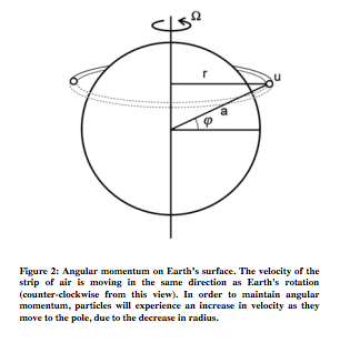
Particles moving pole-ward experience an increase in velocity because of the conservation of angular momentum. In Figure 2, there is a strip of air with velocity u and radius r. If this strip of air were to move upward, the radius would decrease and, in order to maintain angular momentum, the velocity would have to increase.

When air moving pole-ward gets to about 30°, the speed of particles gets to be too fast, and the strip of air becomes unstable, leading to a wavering strip of air as shown in Figure 1. Wind beyond this point to about 60° is very chaotic and unpredictable. The overturning circulation from the equator to around 30° is Hadley circulation, and the chaotic motion is eddy circulation. From this point on, the focus is on Hadley circulation.

Atmospheric Data of Hadley Circulation

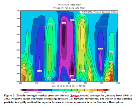
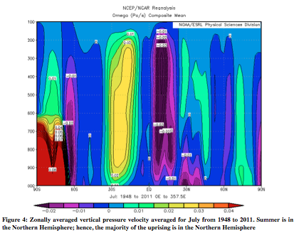
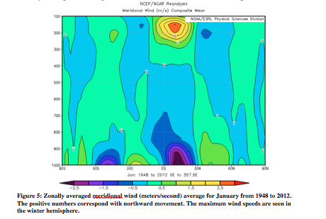
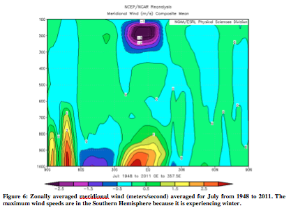
In order to show Hadley circulation in the atmosphere, it is important to show several different atmospheric variables: vertical pressure velocity, potential temperature, and zonal and meridional wind. Following (Figures 3-10) are zonally averaged profiles of these variables averaged from 1948 to 2012 (ESRL). Examples will be given from both January and July. Firstly, Figure 3 and 4 are of vertical pressure velocity, measured in Pascals/second. The uprising occurs where heat is greatest, which results in greater uprising of particles on the side of the equator that is experiencing summer (January – Southern Hemisphere, July – Northern Hemisphere). The air then sets at around 30° on the winter hemisphere, and around 45° on the summer side. As will be seen in all the following atmospheric figures, Hadley circulation is stronger in the hemisphere experiencing winter.

Figures 5 and 6 are of the zonally average meridional wind in January and July respectively. Meridional wind is measured from north to south. Positive numbers represent northward motion. In Figure 5, the greatest winds are observed in the Northern Hemisphere, while it is experiencing a winter. Similarly, in Figure 6, the greatest winds are in the Southern Hemisphere.

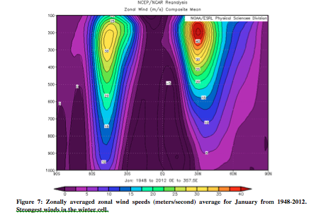
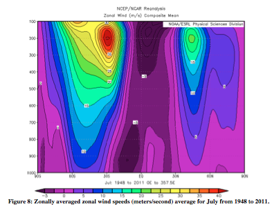
As particles move pole-ward in the upper atmosphere, they get deflected (right in the Northern Hemisphere and left in the Southern). As discussed previously, particles gain zonal speed upon moving pole-ward. Figures 7 and 8 are of this zonal wind speed. The figures also show the trade winds between the equator and 30°, from the return flow at the surface being deflected westward as a result of the Coriolis force.

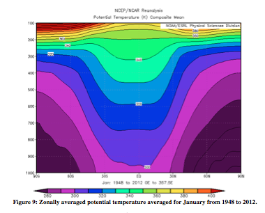
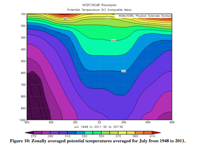
From the thermal wind relation, the greatest wind speeds are associated with the largest temperature gradient. In Figures 9 and 10, the steepest slopes are on the winter hemisphere. In July, there is a much larger difference between the zonal wind speeds of the two hemispheres than in January. This difference is likewise apparent in the July potential temperature data, for which the slope is very clearly steeper on one side.

The two key characteristics of the Hadley cell (from the equator to about 30°) are that there is large-scale overturning circulation, and that wind speeds increase in the pole-ward direction. The next goal was to simulate this in a laboratory environment to study the heat transport associated with Hadley circulation.

Laboratory Experiment

Set-Up

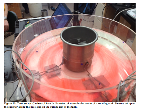
A key characteristic of Hadley circulation is that it is only maintained when velocity is slow. As velocity of air becomes too fast, eddies start to form. In order to simulate Hadley circulation, the rotation rate of a tank of water must be very slow (about 1 revolution per minute); the precise speed was 62 seconds per rotation. The tank was 44 cm in diameter and was filled with 29°C water to a depth of 9 cm. At the center of the tank was a canister, 13 cm in diameter, filled with ice, which was meant to represent one of the Earth’s poles. More specifically, the canister was filled with 415.7 grams of ice, and enough melted ice so that the water level in the canister was also at 9 cm. There were eight temperature sensors total (two sets of four sensors, at 90° apart): 2 on the side of the canister, 2 on the base of the tank at about 2 cm from the edge of the canister, 2 on the base of the tank at 10 cm from the edge of the canister, and 2 on the outer rim of the tank.

Before starting the experiment, the tank of warm water was rotated at about 1 rpm until reaching solid body rotation, which took about 20 minutes. Upon reaching solid body rotation, the ice was placed into the canister, at which point Hadley-like circulation began.

Experimental Results

Basic Motion

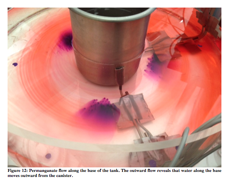
There was sinking of water around the cold canister, outward motion at the base of the tank, rising motion at the rim, and a return flow in shallow water. Figure 12 shows the movement of permanganate, which is a substance that sinks in water. As can be seen, the permanganate moves away from the tank, thus revealing the outward movement of water at the base of the tank.

The overturning circulation described was not the only type of movement observed. In fact overturning circulation such as this would happen in a completely stationary tank. The more interesting observation, from the experiment, shown in Figure 13, was that a dome of cold air formed around the central canister.

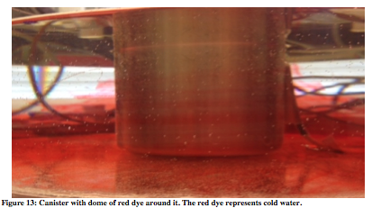
Two simultaneous processes happened to cause this cone to form. There was clockwise sinking of cold water, that moved outward as it descended. Additionally, there was anticlockwise inward rising of warm water. The anticlockwise motion of warm water was in the same direction as the tank’s rotation. In Hadley circulation, westerlies are in the same direction as Earth’s rotation; hence, the anticlockwise motion represents the westerlies. The clockwise motion associated with sinking cold water is similar to the atmospheric easteries.

Heat Transport

In Figure 13, the temperatures of the different sensors are plotted.

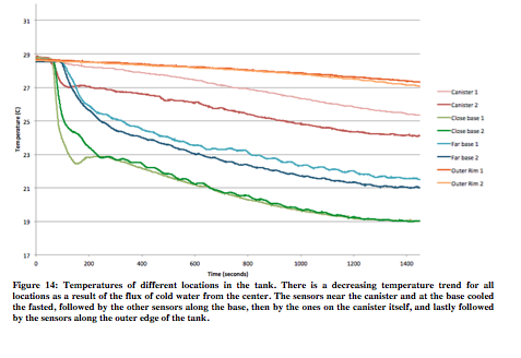
The coldest temperatures were seen at the base of the tank close to the canister. Water sinks near the center and then flows across the bottom of the tank. As such, the sensors at this location will record very cold temperatures. The water along the base but closer to the edge of the tank will be slightly warmer as the cold water interacts with surrounding water, and warms. As water reaches the edge of the tank, it is warmer than the water closer to the tank, and it gets pushed upward. As such the sensors at the outer edge of the tank record the warmest temperatures. Lastly, water will move toward the center of the tank and then sink again, repeating the cycle. As it reaches the ice, the water will sink and cool. The sensors along the canister do not record temperatures as cold as along the base because the water cools significantly before reaching the base of the tank.

Angular Velocity

Below (Figure 15) is the trajectory of paper dots that were placed into the rotating tank. The bottom right side of the figure lacks tracks because the sensors were there preventing the particle tracker from seeing the paper dots.

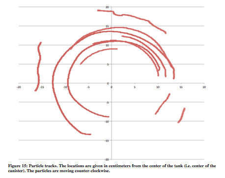
Although none of the tracks made a full circle, it is clear by comparing the radii in each track that the majority of the particles are spiraling inward. Figure 16 shows the angular velocities (in centimeters/second) associated with the inward particle tracks in Figure 15.

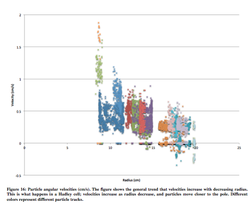
The figure reveals a general trend of increasing angular velocity with decreasing radius. Some negative velocities can be seen for the particles that are toward the edge of the tank, and this is because of the slow speed with which they were traveling. When there is little motion of particles, the tracker may locate the particle a pixel or two off in the wrong direction, thus leading to negative velocities. If this experiment were performed in a bigger tank, or if there was a more accurate way to track the particles, negative velocities as observed in this experiment would likely be less common.

Thermal Wind Calculation

The velocity data above can be compared with the thermal wind velocity prediction. Thermal wind relates wind speeds to temperature gradients. The most reliable place to measure a temperature gradient is along the base of the tank. The equation for thermal wind is:

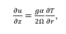
for which α (the coefficient of thermal expansion) is 2.17*10-4 assuming that the average water temperature along the base of the tank is 21°C, g is 9.81 m/s2, and Ω is .101 rad/sec. The difference in temperature between the two sensors along the base was usually 2°, the distance apart was 8cm, and the depth of the water was 9cm. By plugging these values into the thermal wind equation, the predicted difference in speed between the surface and base of the water is 2.37cm/s. Because the temperature gradient chosen was between the two base sensors, this prediction is for the particle speed between those sensors (between 9 and 17 cm radius). The surface particle speeds observed were much smaller than 2.37cm/s, meaning that there was likely a significant clockwise flow at the base of the tank