Introduction
In all thermal systems, imbalances in radiative heating lead to convective or conductive processes in fluid or solid bodies respectively in an effort to evenly distribute heat energy throughout the object. The earth is no exception, and the impetus of myriads of meteorological and oceanological phenomena that exhibit turbulence in this system can often be traced back to attempts of nature to evenly distribute the energy obtained through incident solar radiation.
Conceptual Visualization: The Earth
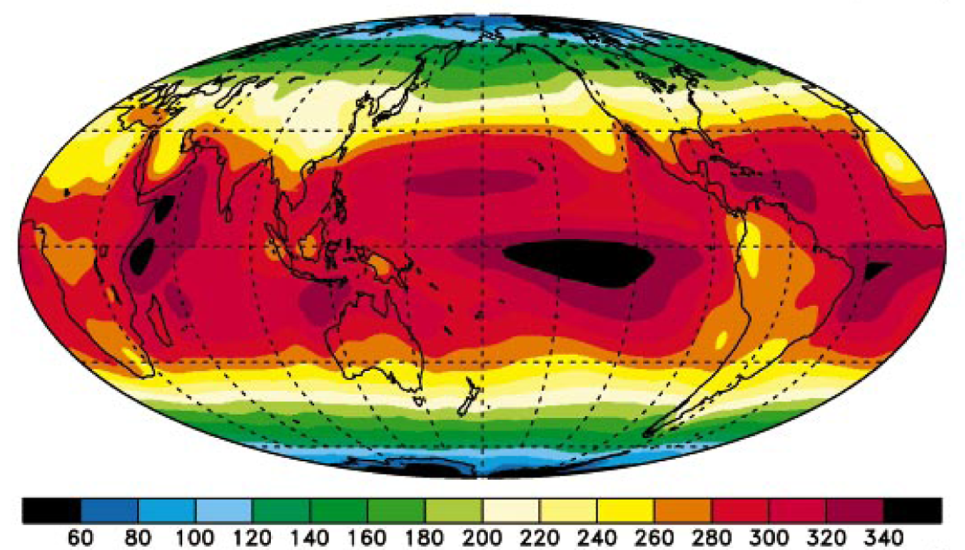
Figure 1.1: Figure from Trenberth and Stepaniak (2003). Copyright 2003 American Meteorological Society (AMS); http://www.climate.be/textbook/chapter2_node6.html
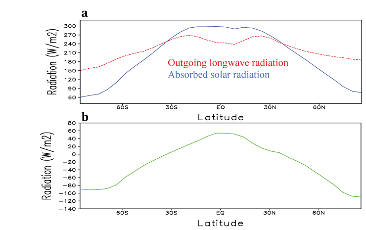
Figure 1.2: Cumulative sum of incoming and outgoing radiation with respect to latitude. http://www.climate.be/textbook/chapter2_node6.html
Given this, it would be sensible to conclude that thermal energy would be transported away from the equator and towards the poles. As such, the concept of the "Hadley Cell" is introduced, as is visible in Figure 1.3. At its root, the Hadley cell is a horizontal circulation pattern that serves as a "conveyor belt" for thermal energy, and significant differences in the cell's behavior can be expected depending on whether or not the fluid is laminar or turbulent. 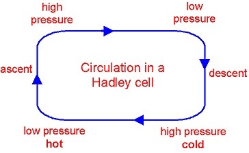
Figure 1.3: At its simplest, a thematic of a Hadley cell. http://www.elgheko.us/meteo.htm
Theory: Laminar or Turbulent Fluid, and Resultant Atmospheric Effects
Given that air should rise near the equator and sink in the vicinity of the polar regions, in a non-rotating system one would expect the motion of fluid to be purely meridional i.e. towards the poles in the upper levels, and away from the poles and directed equatorially at the surface. However, the earth is a rotating system with the atmosphere in roughly solid-body rotation. Therefore, we must take this into consideration by using the Coriolis parameter. Because the Coriolis deflection is weakest at the equator and considering that fluid at the equator orbits the globe where its radius is the greatest, its angular momentum is greater than at any other point on earth since the earth is a solid body. Therefore, by the conservation of angular momentum, we would expect that, to conserve momentum, a parcel of air from the equator attempting to move towards the pole would be deflected eastward in direction since its zonal velocity must increase. Therefore, at the upper levels, a westerly jet should form being strongest as one heads away from the equator. For the sinking air later in its poleward journey, the opposite should be true; as it returns towards the equator, its weakening horizontal velocity due to the increase in radius should lead to surface easterly forming, strongest at the equator. This gives rise to the Intertropical Convergence Zone, where both Hadley cells converge. The rising motion here, coupled with the easterly winds (and the subtropical easterly jet, which, due to surface friction, is considerably weaker than other jets) leads to the development of tropical waves, and is an integral portion of cyclone forecasting.
When the Coriolis parameter is low, the fluid will be mainly laminar, and be governed by the physics of the Hadley cell. However, the entire globe cannot exist as a Hadley cell; proof of this can be sought within the Law of Conservation of Angular Momentum. Given that the radius of a parcel's orbit would be zero at the poles, utilizing solely this law would yield infinite winds aloft at those locations. Given that this is quite impossible, we are forced to rely on eddy heat transport, which "takes care of angular momentum" in other ways by breaking down polar heat transport into more localized vortices. This takes effect at latitudes in the 30-90º regime, where the Coriolis parameter is too great to maintain the laminar nature of the fluid, which results in turbulence. Elsewhere towards the equator, the fluid is largely laminar, leading to Hadley cells becoming the main means of heat transport between 30ºN and 30ºS.
Analogues in the Tank...
Several key differences exist between the earth and our tank experiment; after all, one is a three dimensional rotating sphere comprised of solid, liquid, and gas, complete with pressure gradients amidst the fluid as well as several means of thermal heat fluxes. Meanwhile, the tank is a two-dimensional representation, and the incompressible nature of the water leads to further behavioral differences.
At its root a large rotating cylinder about 0.6-0.7 meters in diameter and 0.25 meter tall acted as a representation of only one hemisphere. Towards the center of the tank, which one can envision "flattening" as a net against the hemispherical form of either the top or bottom half of the globe, a small bucket of ice was placed. The ice was contained in a metal cup with a low specific heat capacity allowing it to efficiently cool the water closest to the center via conduction. As such, a horizontal temperature gradient was formed within the tank, thus allowing the periphery of the tank to become the relative warm "spot" with the fluid rising accordingly, while sinking towards the center of the tank. As the warm fluid rose along the edges, it moved radially inwards where it sank and expanded outwards towards the edges.
One distinction between the tank experiment and the earth is that while the Coriolis parameter changes at each location of the earth (due to a constantly changing angle phi, or the angle equivalent to the earth's latitude), whereas it remains constant in the tank because the Coriolis parameter remains unchanged. Therefore, in order to simulate the change in heat transport regime from being Hadley cell dominated to one tyrannized by rotating eddies, the rotation rate of the tank had to be manually changed. At some threshold of rotation rate, the fluid will transition from being laminar in solid-body rotation to turbulent, resulting in changes in the means of heat transport.
Theory
We can understand the general circulation of the atmosphere by formulating a general theory of the Hadley Cell and its development and progression. Due to the uneven heating of the earth, the equator receives significantly more solar radiation and thermal energy than do higher latitudes. As a result, rising motion and convection occur in this the region known as the intertropical convergence zone (ITCZ). As a result of this rising motion, at the surface air moves equator-ward to replace the air displaced by convection, and air moves poleward aloft before sinking again at about 30o latitude. Thus the formation of the atmospheric "Hadley Cell". Conservation of angular momentum with this northward and southward motion dictates the formation of westerly and easterly winds, and above 30o latitude, a different regime sets in, in which northward flow combined with the Coriolis effect and the thermal gradient with the cold polar regions leads to a more inconsistent regime in which eddies play a major role. The main features of the Global Circulation can be seen below in Figure 2.1.
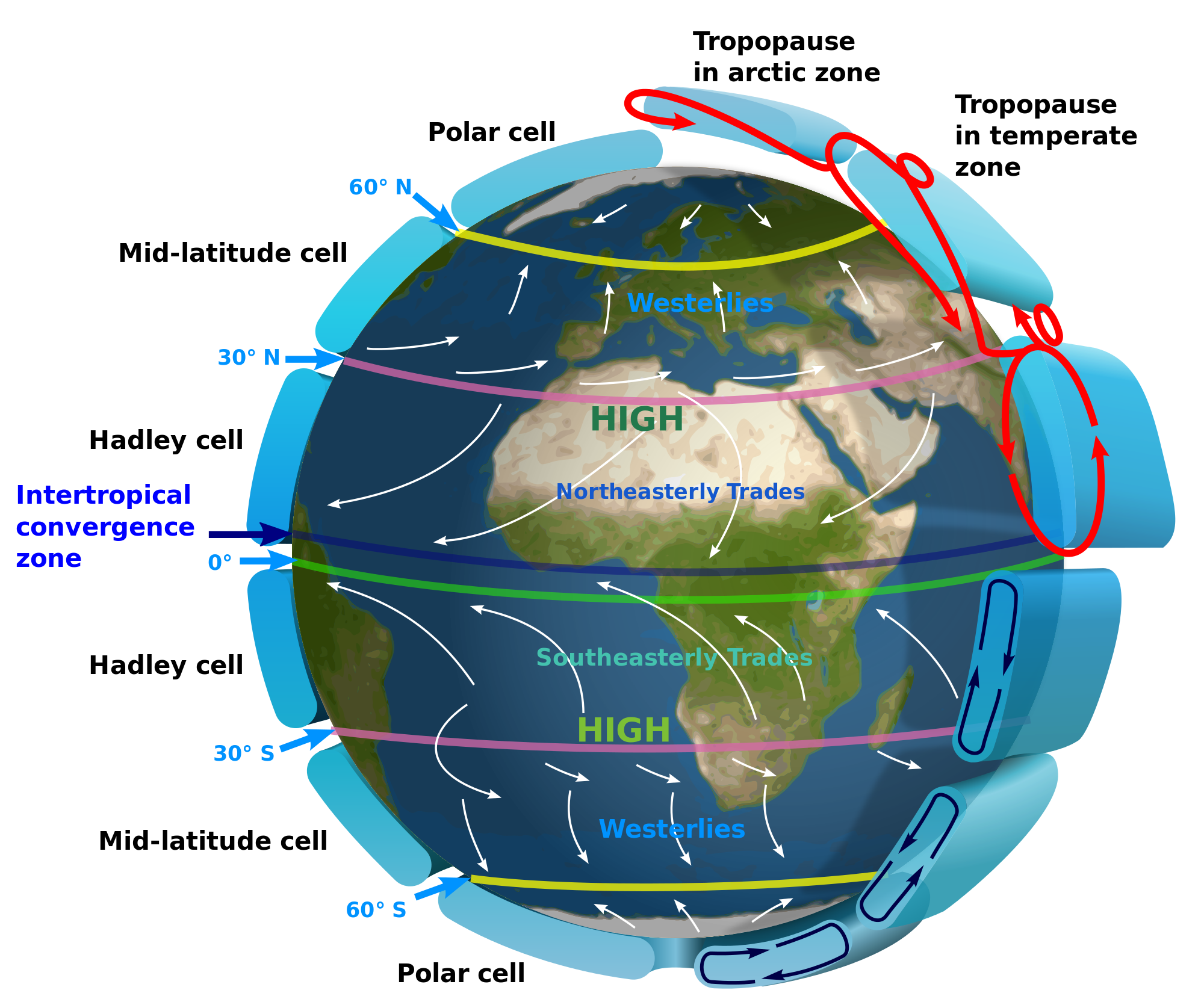
Figure 2.1: The Global Circulation, highlighting both the Hadley Cell and the mid latitude patterns, as well as surface winds.
In the mid latitudes where the Coriolis force is large (unlike in the equatorial regions), the high rotation rate turns what would otherwise be smooth laminar flow, into turbulent flow and the pattern of mid-latitude cyclones, also known as 'transient's or 'eddies', that play an important role in transporting heat from the equator to the pole.
As a result of the Hadley Cell alone, we can observe the formation and location of the subtropical jet stream and equatorial easterly winds, consistent with angular momentum conservation, as seen in Figure 2.2.
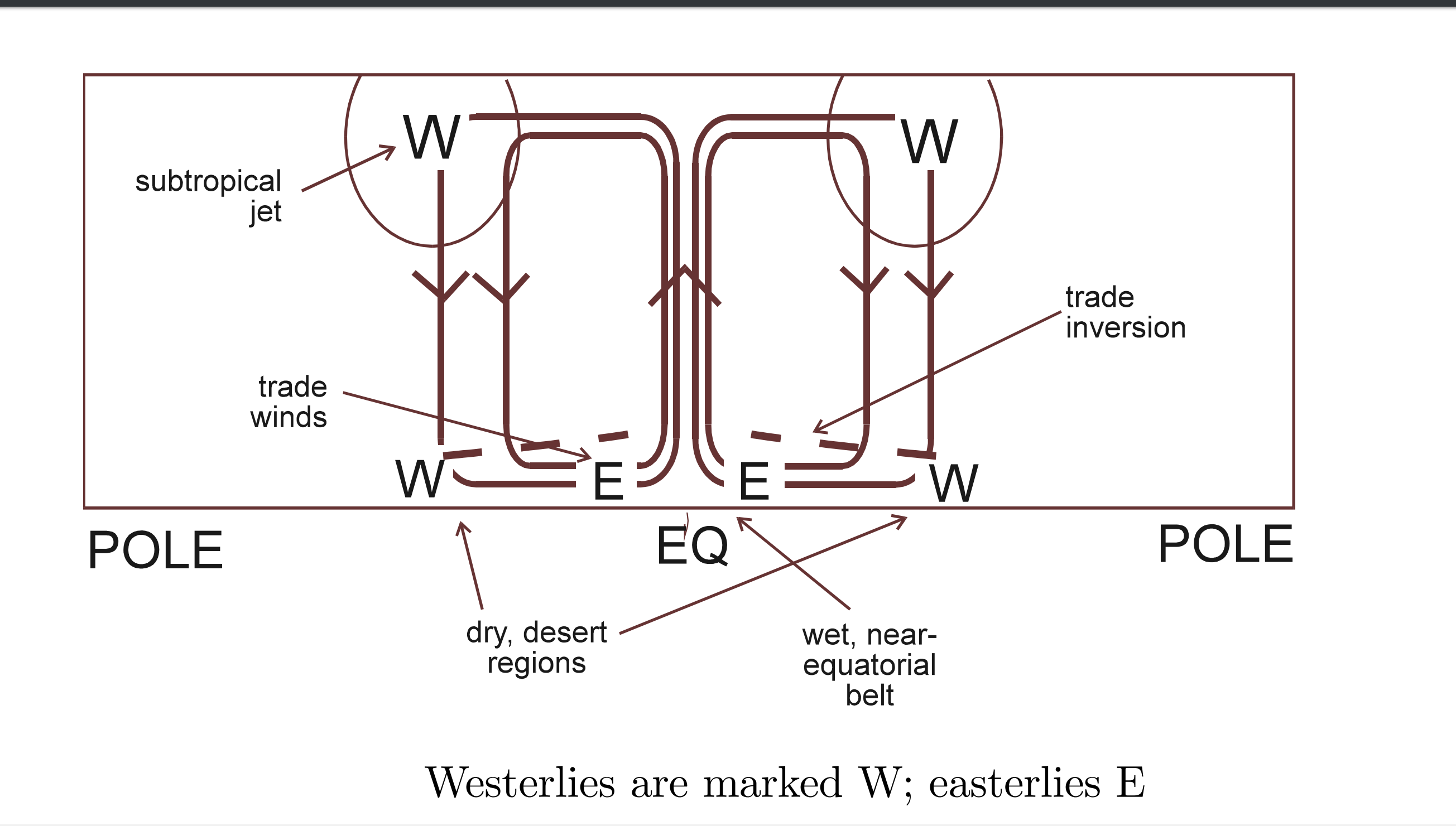
Figure 2.2: The Hadley Cell in cross-section, highlighting both the Wind Patterns that result from it's formation.
In the mid latitudes, poleward motion leads to cyclonic motion under the Coriolis effect. At the boundary between the warmer mid latitude air and the cold polar air, we also observe the jet stream, the increase of wind with height as predicted by the thermal wind Equation 1.
| (1) | $\frac{\partial u}{\partial p} = \frac{R}{fp}\hat{z}\times \Delta T$ |
The instability due to high rotation rates is known as "baroclinic instability", and gives rise to this eddy pattern observed. To balance solar radiation, this eddy heat transport, which dominates, must be on the order of 5x10¹⁵W, which we will attempt to verify with atmospheric data. The equations governing this calculate eddy heat transport as the difference between the mean and the actual heat transport - the remainder. This is defined in Equation 2 as,
| (2) | $\overline{v'T'} = \overline{vT\; } - \overline{v}\overline{T\;}$ |
where the overbar indicate a monthly time average, $\overline{vT\; } $ is the total northward heat flux, and $\overline{v}\overline{T\;}$ is the monthly mean heat transport. Using these we may define the zonal average transient heat flux (zonal heat flux due to eddies) to be
| (3) | $[\overline{v'T'}] = \frac{1}{x_2 - x_1} \int_{x_1}^{x_2} v'T' dx$ |
where $x_2 - x_1 = 2\pi a cos(\phi)$, where $\phi$ is latitude and $a$is radius. Therefore heat flux as a function of latitude may be defined as a pressure integral between two levels of the zonal average, as shown in Equation 4,
| (4) | $\mathcal{H} = 2\pi a cos(\phi) \frac{c_p}{g} \int_{0}^{p_s} [\overline{v'T'\;}] dp |
The equation in the actual yields the curve as a function of latitude displayed in Figure 2.3, compared to the actual atmospheric and oceanic components.
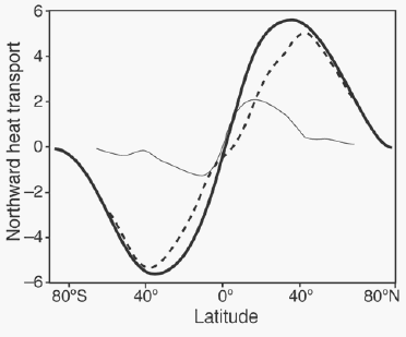
Figure 2.3: Heat flux as a function of latitude, broken up into atmospheric and oceanic components.
As shown in project 2, we expect at the frontal boundary between mid latitude warm air transport and cold polar air, an increase in zonal wind speed with height known as the 'jet stream', that serves both to place a northern bound on efficient eddy transport and maintain the frontal separation. As such we may show in cross section the main features of the global circulation, in Figure 2.4
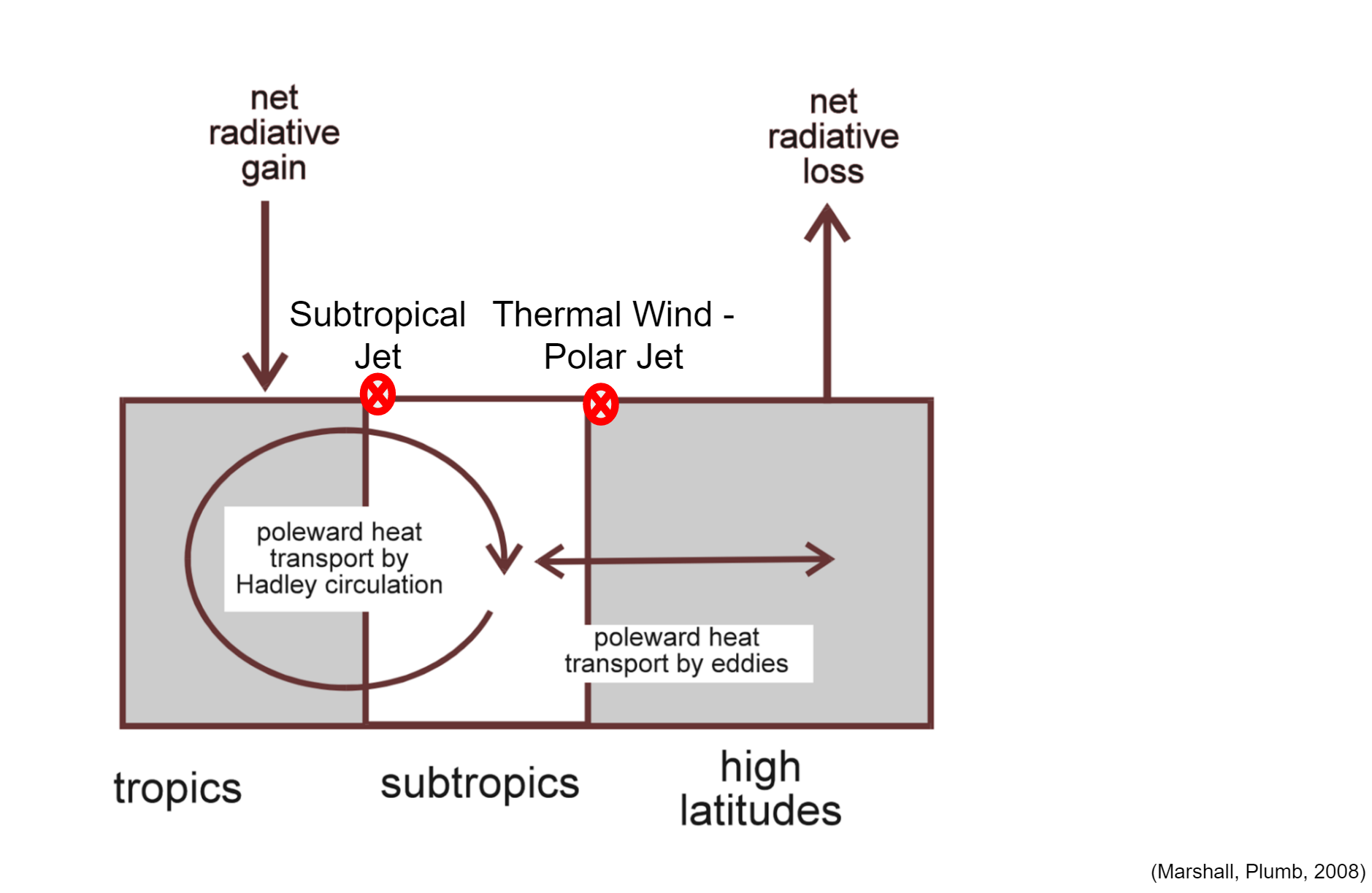
Figure 2.4: A cross-sectional view of the major components of the Global circulation pattern. Note the net radiative influx at the equator and outflux at the poles, balanced by the heat transport in between.
We will use a rotating tank as an an analog to this setup, with low rotation rate mimicking the processes at play in the tropics with low coriolis force, and high rotation rate mimicking the high latitudes. Ice at the center provides the heating imbalance between 'higher' latitudes and 'lower' latitudes. In theory, at high rotation rates, flow will break down and become turbulent. The setup is shown below in Figure 2.5.
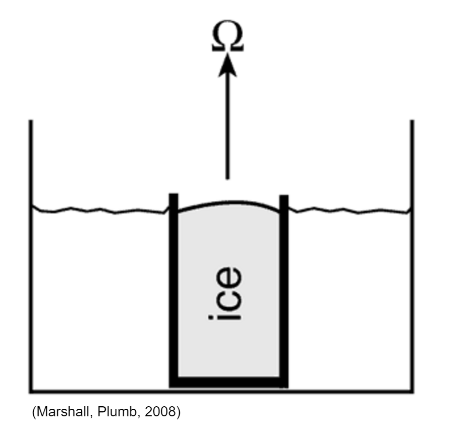
Figure 2.5: The tank setup, showing the tank and ice in cross section across the diameter, with rotation rate \Omegawhich is varied.
In theory, the flow vs height relation for an incompressible fluid with coefficient of thermal expansion \alpha should be,
| (5) | $2\Omega \frac{du}{dz} = \alpha g \frac{\partial T}{\partial r}$, |
where $r$is the radius, and $\frac{du}{dz}$ can be approximated by $\frac{\Delta u}{h} = \frac{u_{top} - u_{bottom}}{h}$, where $h$is the height in the tank. The heat flux, for melting ice, is defined by,
| (6) | $L\frac{dm}{dt} \approx L \frac{\Delta m}{\Delta t} = \rho c_p \int \oint \overline{v'T'\;} dz$, |
where $m$ is the mass and $L$ is the latent heat of fusion for water. Thus the closed loop integral is analogous to a zonal average in latitude, across pressure levels, dz.
The ice heat sink must be balanced by inward radial heat flow, a task accomplished by laminar flow in the low rotation scenario, and eddies in the high rotation case. For the eddies, the Rossby Number may be estimated as a ratio of timescales, or velocity scales,
| (7) | $R_o = \frac{u}{2\pi L}$, |
where $L$ is the length scale of eddy rotation, in meters. Thus we in fact may draw analogs between the tank and the atmosphere, verify thermal wind according to the relation in Equations 1 and 5, and obtain a more complete understanding of wind patterns in the atmosphere.
Laminar Flow in Tank: Analysis and Results
To begin, we first executed the experiment at a low rotation rate to instigate laminar, Hadley cell heat transport. Prior to initializing tank rotation, five thermistors were installed within the tank, as is visible in Figure 1.4:
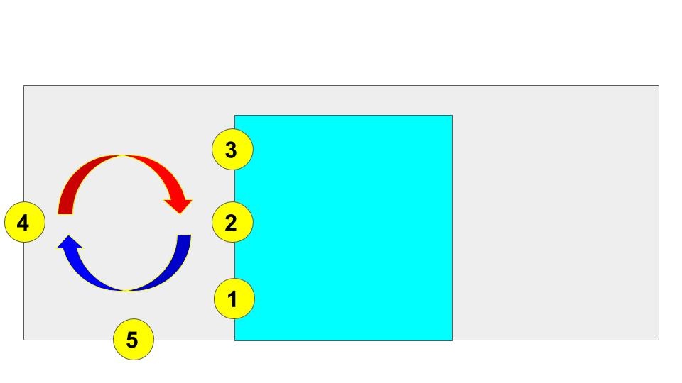
Figure 1.4. (Above)
Given the warming of the water towards the edges (relative) and cooling towards the center as the fluid continued to subduct, one would expect sensor 2 or 3 to report the warmest temperature, whereas the coolest temperatures should be observed at sensor 5. Figure 1.5 depicts the temperatures recorded at each thermistor:
Figure 1.5 (Below)
As expected, thermistors 2 and 3 consistently reported the greatest temperature, while probe five, the deepest, was by far the coolest. This is clearly indicative of the expected behaviors of the Hadley cell. Also noteworthy in the above plot are several "milestones" in the experiment. Since the thermistors were inserted prior to anything else was set up, they recorded the rise in temperature when the water (slightly above room temperature) was added, the insertion of ice into the central container, and the "mixing" of the fluid when the tank was set about rotating.
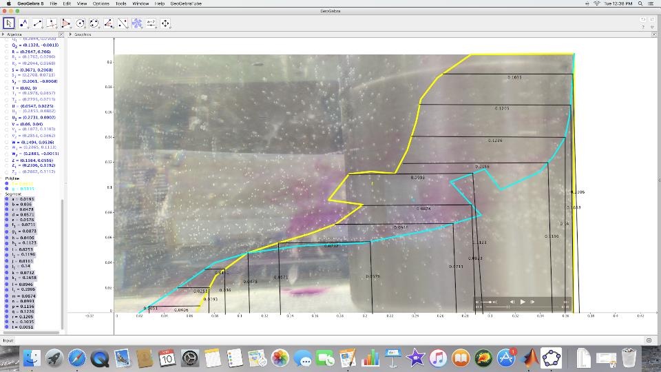
However, in addition to confirming the existence of the Hadley cell in this experiment by means of temperature data, we can investigate the "winds" within the fluid using vertically-dropped permanganate. Figure 1.6 depicts a composite frame of permanganate patterns ten seconds apart, while Figure 1.7 shows a Geogebra photogrammetric analysis of the composite photograph. In Geogrebra, the photograph was scaled so that the axes supplied are in meters. In addition, the yellow line in the latter figure contours the first "snapshot" of permanganate shading, with the blue line marking its position some ten seconds later.
Figure 1.6:

Figure 1.7:
From Figure 1.7 the horizontal distance traveled by the fluid as a function of height may be obtained, allowing one to deduce the translational velocity at different levels throughout the fluid. Figure 1.8 shows this analysis:
Figure 1.8:
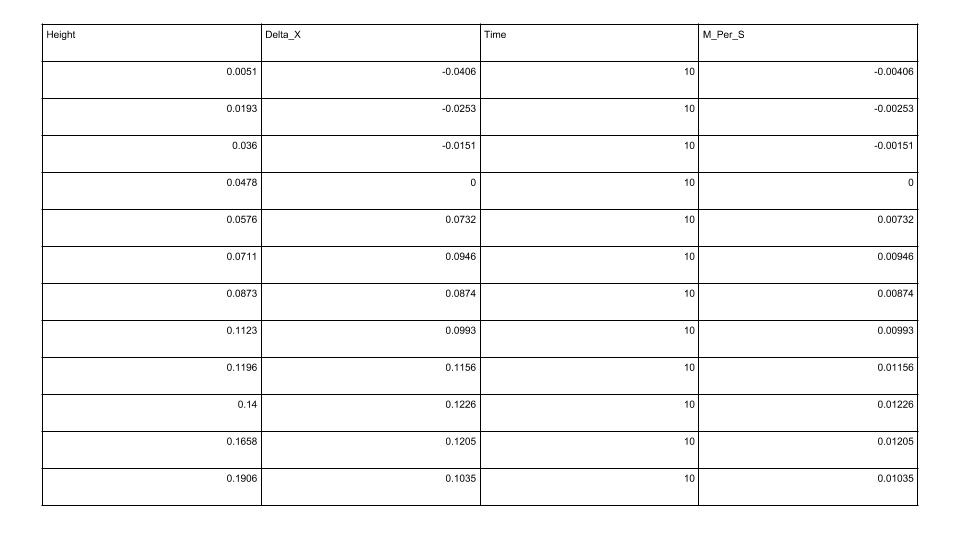
Throughout figure 1.8 the height and the velocity (fourth column) can be seen, and graphed in figure1.9:
Figure 1.9:
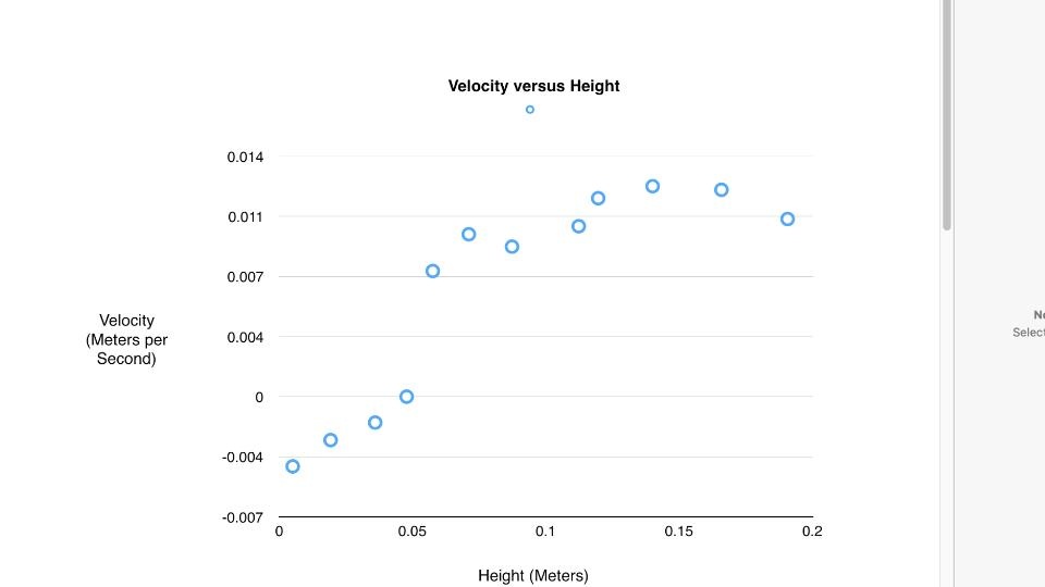
As expected, the velocity begins negative, or directed radially outwards, becoming neutral with height and eventually positive; as one moves towards the vertical extremities of the tank, the maximum positive and negative velocities are found. This is exactly what is to be expected in the Hadley cell. Towards the base of the tank, a weak easterly due to subjecting and "unwinding" fluid and associated frictional drag due to contact with the container's base. Meanwhile, a much stronger westerly developed further up in the tank as water moving towards the center gained zonal velocity due to the conservation of angular momentum.
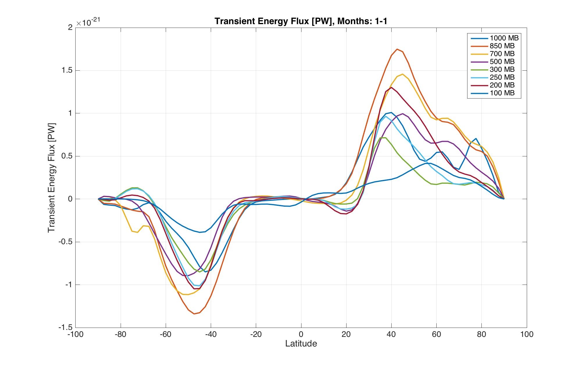
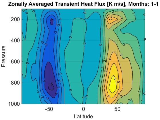
One may notice here that the maximum westerly is not found at the maximum in height. Instead, the maximum westerly wind occurs just below the surface of the water. This is similar to the manner by which the atmosphere behaves; the maximum thermal flux, according to figure 1.92, is visible not at 1000 millibars, but rather at 850 millibars slightly aloft in the atmosphere. In fact, 1000 is the location of the least thermal flux towards the poles. This is a direct result of the behavior of Hadley cells; despite a net positive flux towards the poles, as is necessary, this is where the flux is the least.
Using the above plots, we can confirm the thermal wind relationship using the Margules equation.
Hadley Cells in the Atmosphere
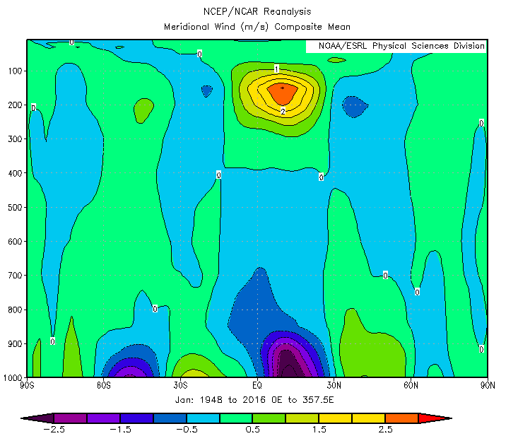
After having developed the idea of an overturning convective cell at low latitudes to transport heat away from the equator and analyzed tank data to develop intuition for the pattern of motion, we will now look at what physical evidence we have for its existence in the atmosphere. The Hadley cell transports heat from the equator to the poles, so we will be looking at wind velocities to see where the net movement is. We know that there is a net north-to-south heat flux, so a good first guess is that this happens via meridional winds i.e. north-south winds. Looking at a plot of meridional wind speed vs. latitude for January, which corresponds to winter in the northern hemisphere, we can see that there are poleward winds at high altitudes and equatorward winds at low altitudes. The plot is shown below with warmer colors meaning a northward velocity direction and cooler colors meaning a southward velocity direction.
Air is being pushed to the pole up high and returning to the equator at the surface, so our initial guess needs to be modified to include how air travels between high altitudes to low altitudes. As seen in our last project, convection is the process that the atmosphere uses to transport heat from the surface to higher altitudes where the heat is then radiated off into space. It makes sense then that a convective plume would exist at the equator, so we must look at a plot of vertical velocity to verify that winds bring air back to the surface at higher latitudes.
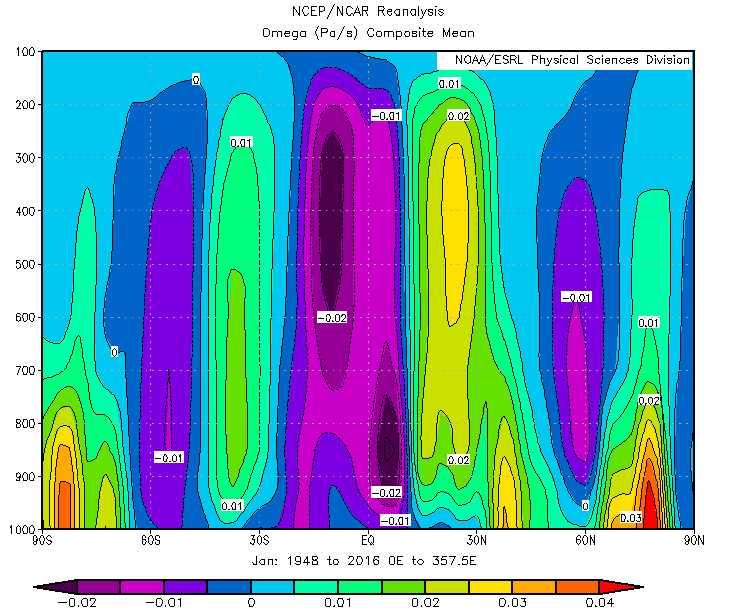
The above graph shows vertical wind velocity. The cooler colors are rising columns, and the warmer colors are sinking columns. While there are adjacent rising and sinking columns spanning the whole surface of the Earth, the strongest winds occur between the equator and 30N. The strongest winds appear in the northern hemisphere because that is where it is winter in January. When it is winter in the southern hemisphere, the strongest columns will be between the equator and 30S. The equatorial column corresponds to convection, and the 30N column corresponds to the point on the Earth at which the warm air has lost sufficient heat and sinks back to the surface. If 30N is the place where warm air becomes cold again, then this is where heat transport stops with the Hadley cell, and as a result, there should be a strong temperature gradient. From our polar front project, we know that horizontal temperature gradients produce a vertical wind shear. Therefore, the place where we observe the strongest temperature gradient should be where we see the fastest increasing winds and the greatest overall wind speed. Looking at the following plot of zonal (i.e. west-east) winds, the greatest wind shear and resulting wind speed occurs at 30N, where the greatest horizontal temperature gradient is and where the air in the Hadley cell cools off again.
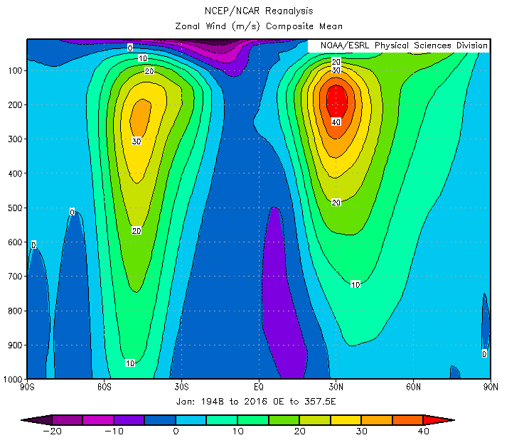
Superimposing the three graphs of wind speed on top of each other, we can get a general picture of how winds move in the Hadley cell between the equator and 30N. Air rises at the equator due to convection, is transported northward to compensate for the meridional heat imbalance, cools off at 30N where the greatest temperature gradient is, resulting in zonal winds and also the sinking of now dense air and resulting equatorward movement to compensate again for the meridional heat imbalance.
We have now shown that what we expected, an overturning cell at low latitudes to transport heat to the mid-latitudes does in fact exist and we can see it by inspecting wind velocity vs. latitude in the atmosphere. The Hadley cell is only responsible for heat transfer to the mid-latitudes, so there must be some other mechanism to bring heat from the mid-latitudes to the pole. The farther away from the equator we go, the more important the Coriolis parameter is, and small-scale eddies or rotating weather systems will be the main mechanism for heat transport. To understand what this looks like, we will conduct our tank experiment again except at a faster rotation rate to make a link to the higher latitudes.
Eddy Heat Transport in the Tank
In the tank experiment mentioned above, we looked at how water moves between the outskirts of the tank and the center where the ice bucket is to transfer heat. A rotation rate was chosen to create movement most similar to the Hadley cell, but we conducted the experiment again except at a faster rotation rate to create movement most similar to eddies. Likewise, four thermistors were placed in the tank when the rotational speed was increased and thus the Coriolis parameter augmented to a point when the regime would shift to one of eddy heat transport. Figure 2.0 illustrates the positions of said thermistors:
Figure 2.0: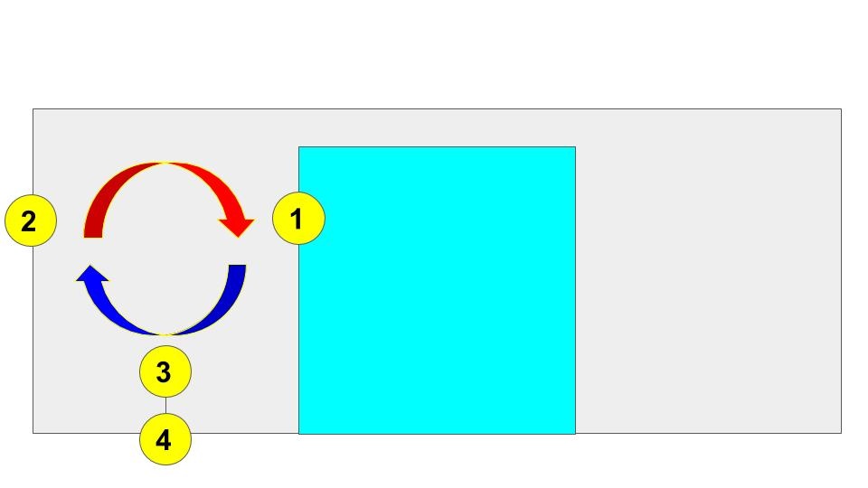
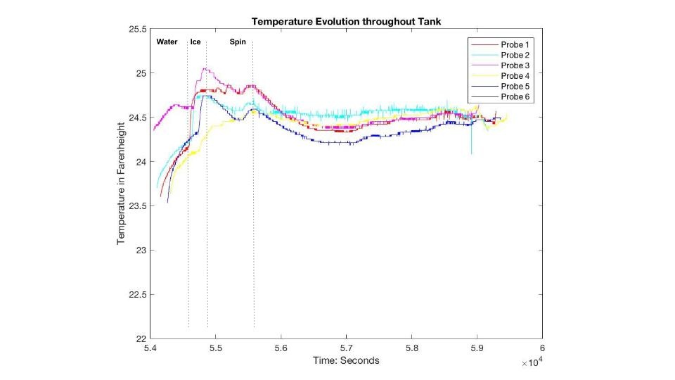
It would be anticipated that the greatest temperatures would be found at thermistor 1, and the coolest in turn at thermistor 3 or 4. Figure 2.1 depicts the trace of thermistors' reports during the duration of the experiment:
Figure 2.1:
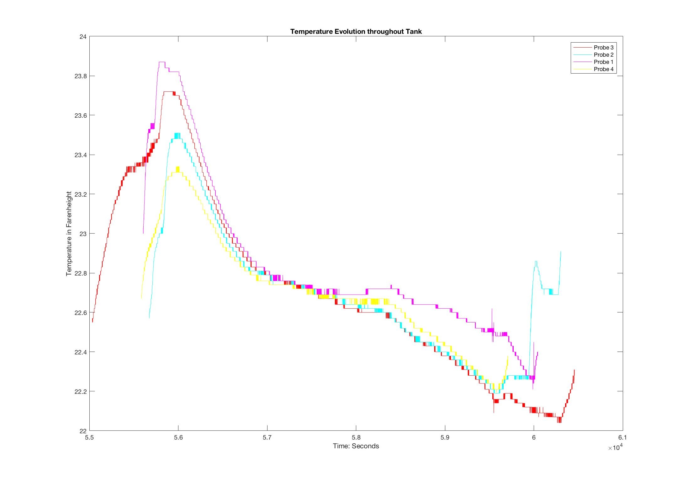
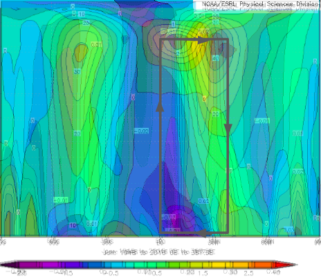
Though difficult to discern due to the technical limitations of Wiki, it becomes clear that the warmest temperatures were, in fact, recorded at thermistor 1, with the chilliest readings located at thermistor 3. This is exactly what would be expected. Unlike the gentler slope within the laminar fluid, however, the eddy transport nature of this second trial of the experiment lead to an oscillating, varying "stair step" pattern in temperature measurements. In addition, an effort was made to determine the velocity of different points using the particle tracking software; the positions of the points sampled is shown in figure 2.2:
Figure 2.2:
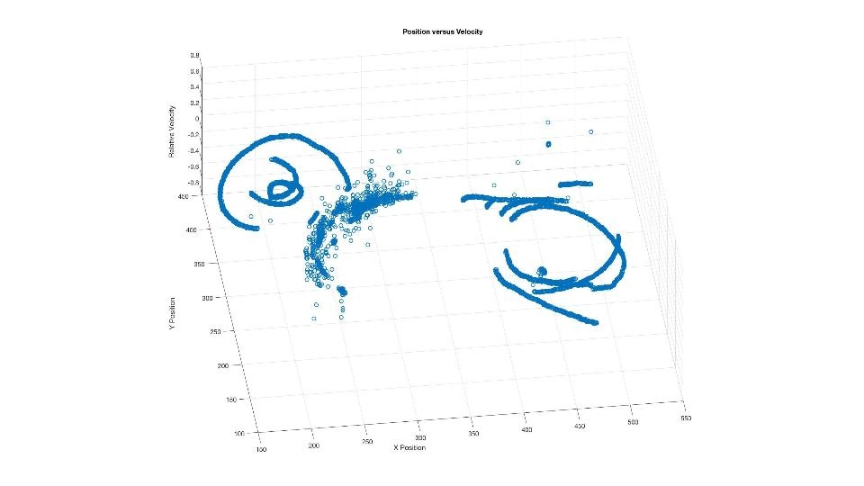
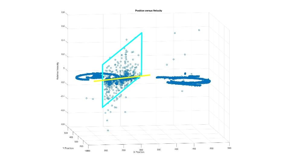
The most dramatic eddy sampled using the particle-tracking software, visible in part on bottom left-hand side of figure 2.2, is quite telling apropos to the "heat flux" within the tank. Despite rotation throughout the eddies towards and away from the center, the thermal gradient within the tank suggests that heat should have a net movement towards the center. A side view of the same graph focused on the most intense eddy illustrates the "winds" embedded within this rotating swirl of fluid; positive velocities are towards the center, with negative velocities away from the center. At first a chaotic scatter of points demarcating velocities at given points (with the x and y axes marking position, with the z axis reserved for velocity), a blue parallelogram has been drawn into Figure 2.3, along with a yellow line illustrating the zero level of velocity from the graph's perspective. One can clearly note that the area of the parallelogram containing data points above the zero line is far greater than below the line, indicating a net movement towards, and thus a heat flux in the direction of, the center. This is exactly what is expected in the atmosphere, and what our group observed in the tank.
Figure 2.3:
 In addition, our group was able to note at least half a dozen eddies embedded within our fluid visually using food coloring and dye; the red was placed on the outside of the tank, with blue inside the tank. As mixing occurred, the dyes were dragged along with the rotating fluid, and as such the patterns of warm and cold water were able to be shown. Figure 2.4 depicts these illustrative markings:
Figure 2.4:
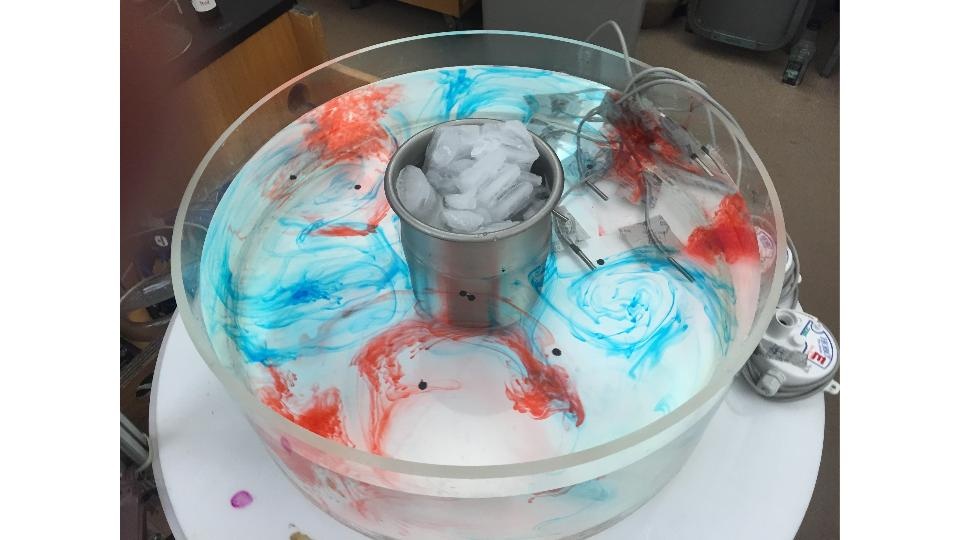 Thinking back to Project 2, an investigation into the thermal wind balance and formation of the jet stream, one could in essence convert the motion of particles throughout the fluid into a vector field; in doing so, there would exist one continuous path that completely encircles the central cold-dome within the tank. This would indicate the jet stream, with the serpentine pattern waving towards and away from the center and ensnared within eddies and vortices rotating around in the larger body of fluid. One may note that the blue and red eddies rotate in opposite directions, much as is the case within the atmosphere due to regimes of higher and lower pressure.
One item of note in figure 2.1 is that the temperature at each sensor, though subject to slight oscillations due to eddies, slowly decrease with time somewhat uniformly throughout the fluid. This is to be expected, as the thermal energy contained within the relatively warmer is transferred and over time reduced as it in turn warms the ice to above melting point. Thus, though the temperature of the ice/water solution remains at 32 degrees, the increased thermal energy is instead utilized in the form of latent heat, responsible for the change in phase of the liquid. As such, the amount of energy needed to fully melt the block of ice placed in the center should be equal to product of the ice's mass and the specific heat of fusion. Therefore, considering that 771.4 grams of ice were used in the experiment, one would anticipate that roughly 258,000 Joules of energy would be necessary complete this thermal transaction. Spread over a period of approximately 4,000 seconds, the result is in effect the energy required to power a 64-Watt light bulb, and may be practically thought of as a "negative light bulb" placed in the center of the tank according to Dr. John Marshall. An example of a 65-Watt bulb is depicted in figure 2.5.
Figure 2.5:

Eddy Heat Transport in the Atmosphere
The tank experiment showed us that small-scale rotations are responsible for transporting heat when the rotation of the Earth is important enough as is the case at sufficiently high rotation rates and high latitudes. We will now look for evidence that heat is transported via these eddies or transients as they are called since the systems last for a finite amount of time. Below is a map of the surface of the Earth plotted with transient heat flux. Yellow contours mean northward heat flux, and colder blues mean southward heat flux.
To get a clearer sense of the transient heat flux dependence on latitude, we will take a zonal average i.e. average over all of the longitudes.
With this graph, the general trend of transient heat flux being directed poleward is evident, and the total transient heat flux can be quantized by summing over all pressure levels in the next figure.
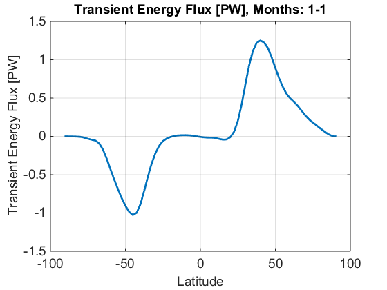
Here is a quantitative graph of transient heat flux at different latitudes. Notice that the zonally averaged heat flux map shows that the maximum transient heat flux is ~6 PW, and this graph only shows 1-1.5 PW. A possible reason for this is the fact that the data set filtered out weather systems that were shorter than two weeks. We can also look at the transient heat flux for each pressure level, which shows that the most heat is transferred just above the surface at 850 mb.
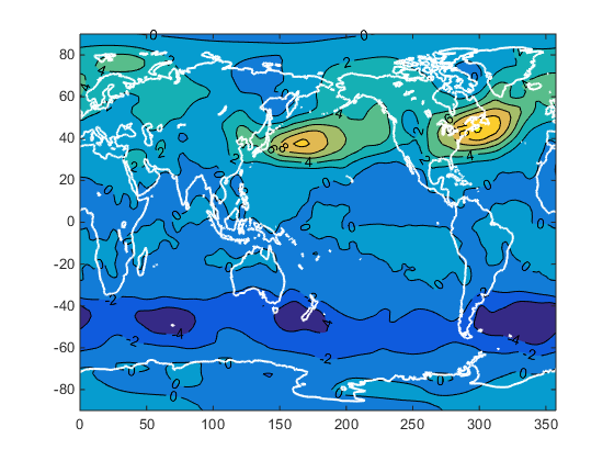
Using NCDC's and NCEP's data, the Transient Energy Flux across different levels of the atmosphere in January can be plotted with relative ease. As previously mentioned, the Coriolis parameter of the earth only supports the Hadley cell between 0 and 30º on either side of the equator. As such, the remainder of the globe is dominated by eddy heat transport.
Because January features winter in the northern hemisphere, a stronger temperature gradient leads to a more significant poleward heat transport than in the southern hemisphere. This is evident in our findings, given that the peak at northern latitudes in flux is far greater than in southern latitudes. The Hadley cell theory is also supported by the weak positive flux at the surface (1000 millibars) between 0º and 30º north. This is because there is a weak easterly with a slightly northerly component as air returns radially towards the equator; theoretically, there could be negative flux, but some "mixing" of northerly winds likely aids in some weak northerly flow near the surface. The majority of the heat transport occurs aloft, but the heat flux which measures the amount of heat transport at various levels, should be directly proportional to height (for obvious reasons described previously under the theory of Hadley cells) and pressure (as denser air can carry more heat per unit area). Therefore, the location of the "maximum" should be the "happy medium" between height and pressure, which we would estimate to be located around 700-850 millibars, as revealed by the graph. This is coincident with the jet stream, which is essentially the a narrow band of intense westerlies. In addition, the rising air characteristic of the Intertropical Convergence Zone at the equator is tempered by a weak high pressure dome aloft, which can be seen in the extremely weak flux towards the equator at the uppermost levels of the atmosphere. In addition, it was previously mentioned that friction with the surface would reduce the flux close to the ground, which is supported by the lower level of flux at the 1000 millibar level.
Figure 1.92:
(Please do note that the Transient Heat Flux in Petawatts should not feature a 10^-21 factor; that should be omitted).