Midlatitude Eddy Circulation

Hi! We're Elizabeth, Elizabeth and Katrina, and here's our write-up of the midlatitude eddy circulation portion of our general circulation project.

Introduction

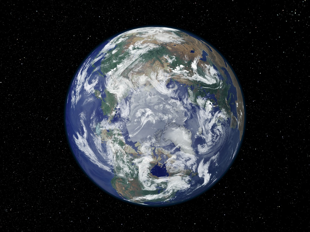
Source: http://visibleearth.nasa.gov/view.php?id=56236

The midlatitude eddy circulation, which we can observe surrounding the pole in the satellite image above, is important for heat transport in the atmosphere. Eddies occur at higher latitudes than the Hadley Cells and as estimates in the plot below show, are responsible for most of the heat transport required by the differential heating of the Earth. Once again we used a tank experiment and atmospheric data to study these eddies. Eddies occur in the midlatitudes, where Earth's rotation is more significant. Thus, to mimic eddies in our tank experiment, we used a high rotation rate and temperature gradient. To study eddies in the atmosphere, we used atmospheric data to study the heat transport involved in the midlatitude eddies.

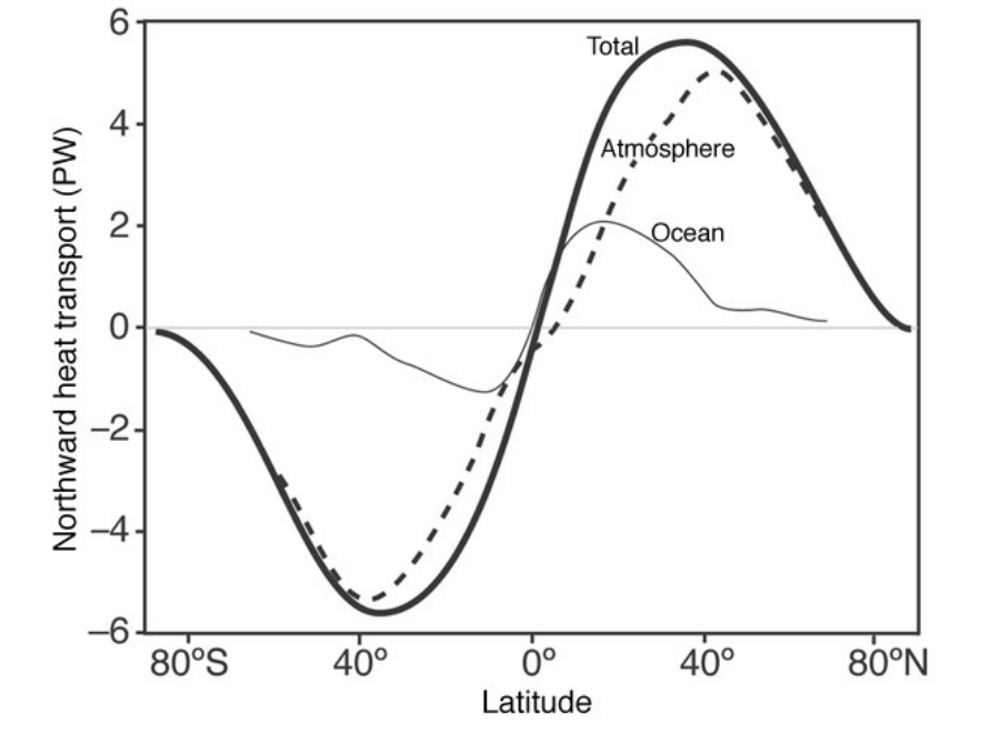
        Source: "Atmosphere, Ocean, and Climate Dynamics: An Introductory Text" by John Marshall & Alan Plumb (2007).

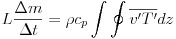
From the figure above, detailing heat transport by latitude, heat transport is at a maximum near 40ºN and S, where eddies occur. We integrate the zonally averaged heat flux due to eddies, to find the net poleward heat flux using the following equation,

where a is the Earth’s radius, is the latitude, c_p is the specific heat, g is gravity, and  is the zonal average of , with v referring to meridional wind and T referring to temperature. Here,  is the total heat flux and  is the monthly mean transport. Thus,  is the meridional heat flux due to transient eddies; using this equation we will compare its result to what the figure above predicts. 

Atmospheric Data

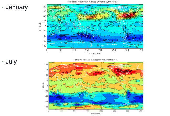
We can notice a couple interesting things from these plots. In the January when the Northern Hemisphere is experiencing winter, we see two clear maximums of Northward heat flux. These could be because the temperature gradient is strongest during the winter. The maximums are located on coasts where there are strong land-sea interactions. The combination of the stronger gradient and land-sea interaction could result in more synoptic scale storms and more eddies, resulting in stronger heat flux in those regions. In July when the Northern Hemisphere is experiencing summer, we observe that the northward heat flux is stronger overall in the Northern Hemisphere as well as more uniform. In both January and July, we see strong southward heat flux in the Southern Hemisphere.

We next plotted the zonally averaged transient heat flux, averaged over the longitudes following:

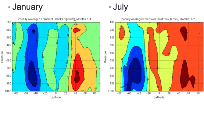
These two plots again show poleward heat flux in both hemispheres. Both plots also show two maximums of heat flux, one at a higher and one at a lower altitude. Maximums in heat flux can be caused by either differences in velocity or in temperature. Higher in the atmosphere, the heat flux maximum could be driven by the strong velocity difference around the fast polar jet. Lower in the atmosphere, the heat flux maximum could be caused by the difference in temperature between the land and ocean.

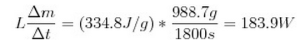
Finally, we vertically integrate the zonally averaged transient heat flux and multiply by some constants to find the zonally and vertically integrated transient sensible energy flux using:

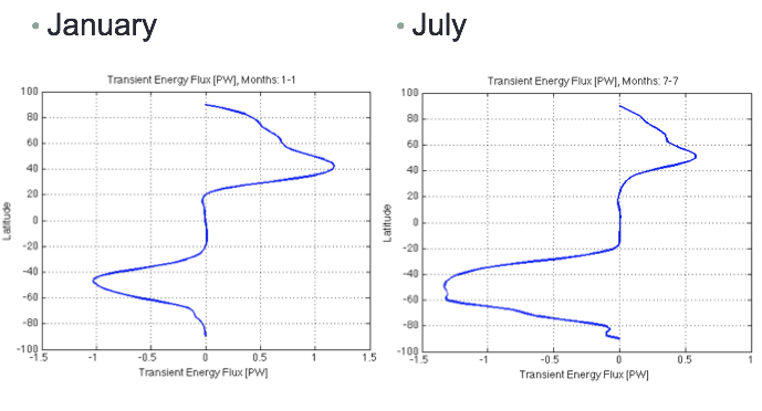
The maximum energy flux away is approximately 1PW and found around 40ºN and 40ºS because the eddy heat transport carries heat from the midlatitudes to the poles. The maximum energy flux from the atmosphere is actually about 4 PW in both North and South directions from around 40ºN and 40ºS. There is a discrepancy because we only calculated the sensible heat energy flux, neglecting the contributions from latent heat energy and potential energy that contribute to the 4PW plot.

Tank Experiment

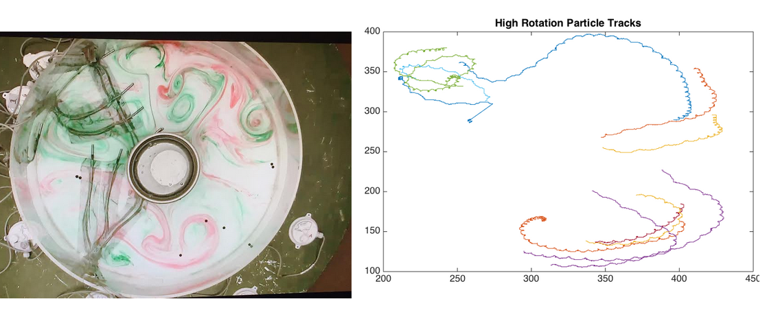
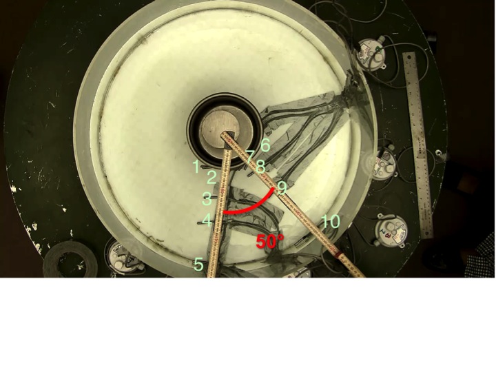
Using a high rotation rate (10 rotations per minute) to simulate the much higher Coriolis parameters at near-polar latitudes, we set up a tank experiment to observe eddy heat transport. As in the Hadley experiment, a metal bucket of ice was placed at the center of a rotating circular tank. However, due to the high rotation rate, dots placed on the surface of the water were observed to follow the shape of smaller-scale eddy currents, rather than rotating around the tank. Similarly, red and green dye placed in the tank highlighted small disturbances and rotating cells.

As in the Hadley cell experiment, a temperature gradient was observed to have developed much more strongly at the bottom of the tank, due to the denser, colder water sinking downwards.

 

The 988.7 grams of ice were not replenished over the course of the experiment and took thirty minutes to fully melt. Assuming that the power outputted by the ice was equal to the heat transported by the eddies, the system could be described by the following equation:

 

where L is the latent heat of fusion, m is the starting mass of the ice, t is the time it took to melt, ρ is the density of water, cp is heat capacity, and v’ and T’ are the variance in velocity and temperature, respectively. Unfortunately, we had difficulties calculating v', so we used .6 mm/s, the value cited on the PAOC website in our calculations (http://paoc.mit.edu/labguide/circ_exp_fast.html). While inaccuracies in the measurements and the fact that we could not place thermometers over the entire tank led to some imprecision, we would still expect the right and left sides of the equation to agree within approximately an order of magnitude. Calculations can be found below:

 

RHS

LHS

 

The two sides of the equation are off by a factor of three, which is a close enough agreement to confirm that the relation holds. The discrepancy may be due to a couple of factors. We had some delays starting the experiment,which meant that the ice started to melt and the starting mass may have been much less than 988.7 grams. Additionally, the velocity variance value was taken from a different experiment, so it's likely somewhat off from the value we would expect in our experiment.