The Dynamics of Fronts - Dig Deeper May 2019

By: Bea Nash and Bethany Cates

1 Introduction

For our Dig Deeper Project, we build on our work from Project 3, in which we examined the general flow dynamics created by the interaction of fluids of different air masses. In Project 3, we modeled the resulting circulation as a two-layer system, but we did not consider the shape of the boundary and how it affects the flow. Fronts, the boundary between these masses, are really important for weather systems - most everyday weather phenomena occur at frontal boundaries. In this experiment, we investigated the frontal boundary more closely: we first introduce two experiments designed to replicate two different types of fronts (atmospheric and oceanic), then discuss fronts in both the atmosphere and ocean.

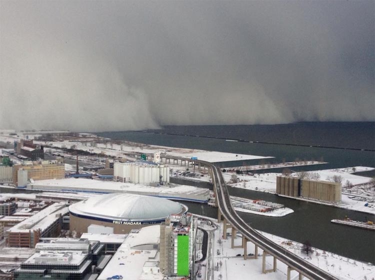
Figure 1.1: Sharp frontal boundary in Buffalo, New York. Thick clouds and precipitation often accompany cold fronts.1

2 Tank Procedure

We created two versions of this experiment. We will discuss the second version in section 5. For the first version (hereafter "the regular dome version"), we first placed a bottom-less cylinder (in our case, a paint can) dead center in a circular tank, sealing the edges of the cylinder with vaseline to prevent water escape. We then mixed our salty liquid: we added kosher salt to several gallons of water (most of which would be used in the next version of the experiment) until we reached a final density of 1.03 g/mL, contrasted with the freshwater from the tap at 0.94 mL.

We then filled the center cylinder with the salty fluid, and added several drops of green dye. (We should have added more drops, because it was actually quite difficult to see the dome after the cylinder collapsed!) We then spun the tank up to solid body rotation at 8rpm, and carefully lifted the cylinder vertically out of the water, trying to add minimal disturbance to the system (see Figure 2.1).

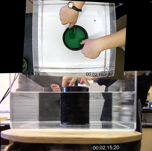
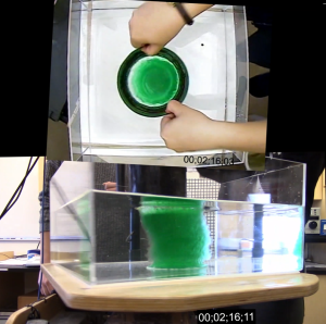
Figure 2.1: The moment just before (left) and after (right) removing the cylinder from the tank. You can already see the cylinder beginning to collapse in on itself.

After removing the cylinder and allowing the system to settle for a bit, a dome formed in the center. Because we hadn't added much dye, it was difficult to see the shape of the dome. We added a few more drops of dye, as well as a few handfuls of neutrally buoyant floats, to trace the frontal surface. We then dropped several paper dots on the surface of the dome.

3 Background theory: Thermal Wind and Margules relation

We can explain the flow at the surface by drawing on our knowledge of the geostrophic and thermal wind relations from project 3. Any time there is a temperature difference between two air (or in the lab case, fluid) masses, there is a pressure gradient force. When the system is in geostrophic balance, the pressure gradient force is balanced by Coriolis forces. For the purposes of this derivation, we assume the system is in geostrophic balance - maybe not the best assumption on a turntable of this size rotating at 8rpm!

We would expect a wind aloft perpendicular to direction of the pressure gradient even if the isosurfaces are parallel. When the isosurfaces are not parallel, however, the pressure gradient force changes with height; the larger the slope of the isosurface relative to the Earth's surface, the larger the pressure gradient force. Likewise, the large the pressure gradient force, the larger the resultant geostrophic wind (see Figure 3.1). The change in the geostrophic wind as a function of height is known as the thermal wind.

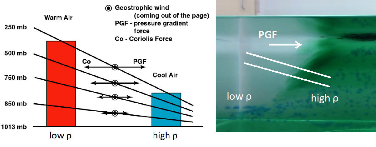
Figure 3.1. Because the vertical distance $\begin{array}{l}\Delta z\end{array}$ between isosurfaces is consistently larger for the warm air, the pressure gradient force increases with height. The analogous situation in the lab is shown. 6

So we have an understanding that the slope of a frontal surface directly corresponds to the pressure gradient force, in turn affecting the magnitude of the geostropic wind. We'll now try to use this knowledge to derive a relation between the slope of the dome and the speed of the particles circulating at the surface.

In order to predict the frontal slope, we first find the change in pressure along two different paths: one through the dense fluid and the other through the light fluid, both with the same start and end point. Since they have the same start and end point, we require that the change in pressure calculated along these paths must be equal (see Figure 3.2).

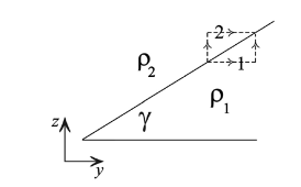
Figure 3.2: $\begin{array}{l}\rho_{1}\end{array}$ is the denser fluid, $\begin{array}{l}\rho_{2}\end{array}$ the less dense fluid. γ is the angle between the denser fluid and the bottom of the tank. We calculate the changes in pressure along paths 1 and 2 and require that they be equal.2

Next, we assume that the flow is in geostrophic balance:

$\begin{array}{l}\large{u = -\frac{1}{\rho}\frac{\delta p}{\delta y}}\end{array}$ (3.1)

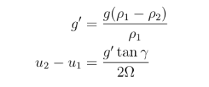
The result is the following relation (Margules relation) for the slope of the frontal boundary:

(3.2)

where γ is the angle the dense fluid makes with the horizontal, $\begin{array}{l}u_{2}\end{array}$ , $\begin{array}{l}\rho_{2}\end{array}$ are the azimuthal velocity and density of the less dense fluid, respectively, $\begin{array}{l}u_{1}\end{array}$ , $\begin{array}{l}\rho_{1}\end{array}$ are the azimuthal velocity and density of the denser fluid, and $\begin{array}{l}\Omega\end{array}$ is the rate at which the system is rotating, in radians/second.

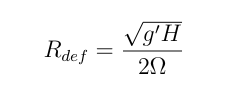
Assuming that angular momentum of the fluid is conserved (only a valid assumption when friction is negligible), we get the following relation for the (approximate) deformation radius:

(3.3)

where H is the height of the free surface with respect to the bottom of the tank.

The deformation radius gives an idea of how much the front will spread before reaching a stable state. In the subsequent section, we discuss how well these theoretical predictions align with the results of our laboratory experiments.

4 Lab results

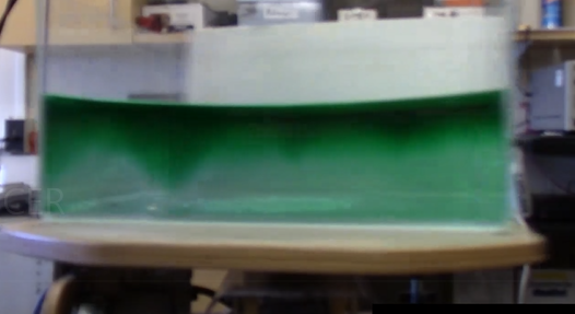
In order to collect data from our experiment, we track the motion of buoyant particles at the surface of the fluid, as well as particles with density in between that of the two fluids which sat just above the frontal boundary. The shape of the front, although relatively stable, did vary slightly throughout the course of the experiment, as can be seen from the following images.

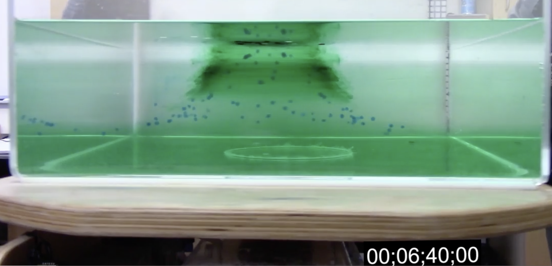
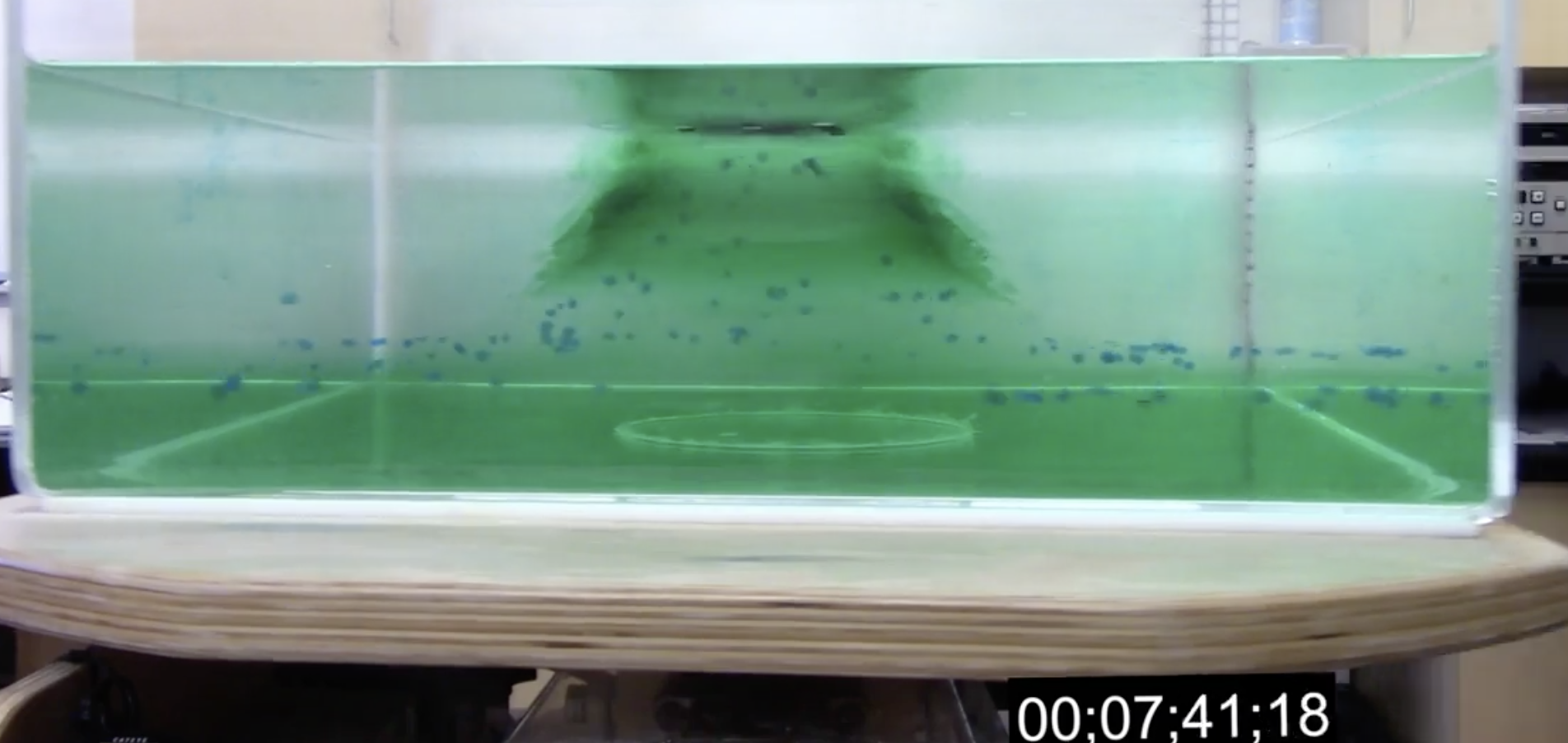
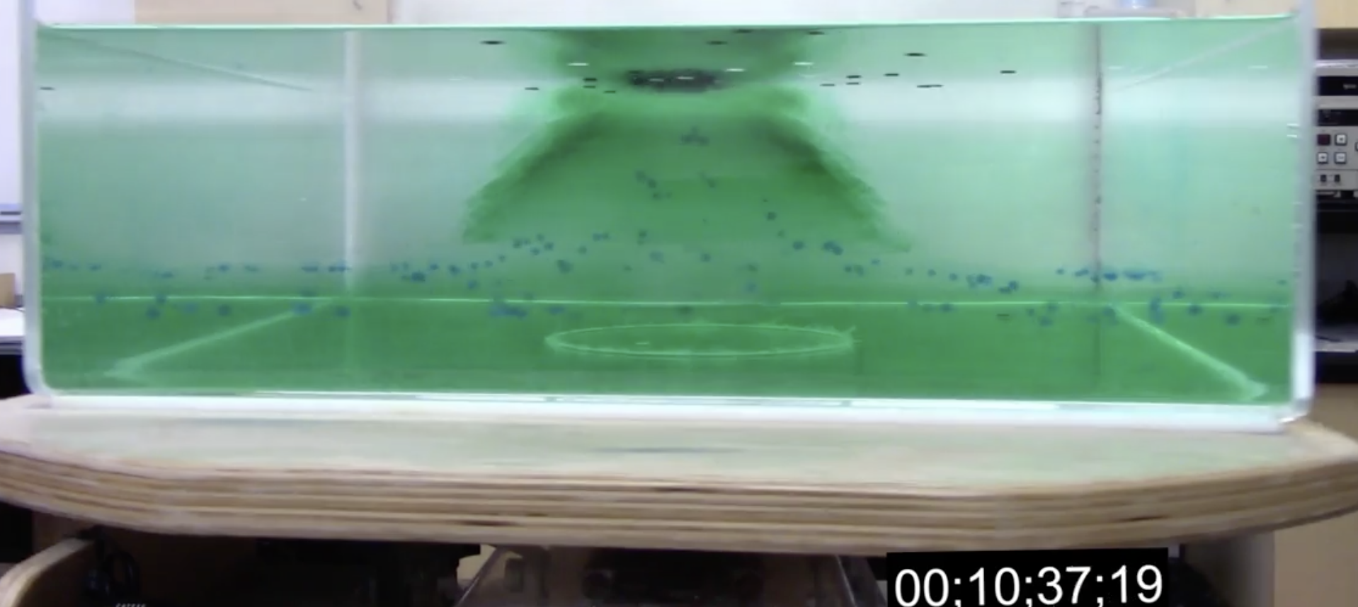
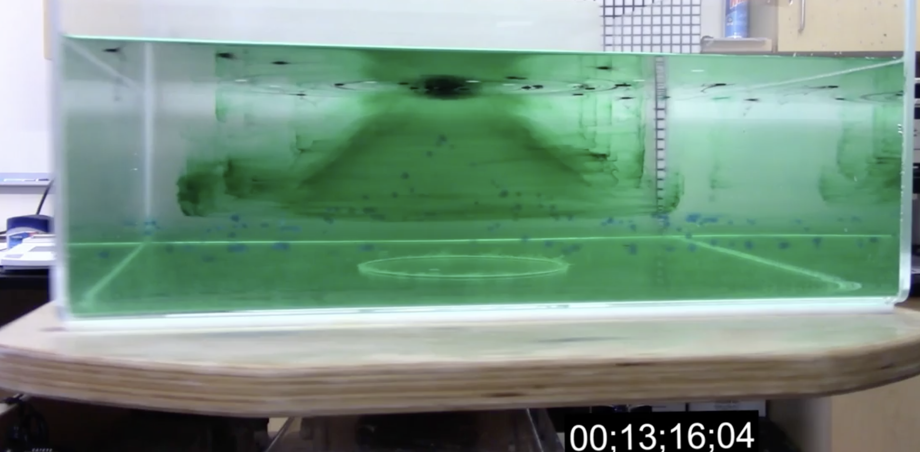
Figure 4.1: The progression of the front. The time stamp shown is relative to the time at which the can was removed. The green dye is placed just outside the frontal boundary and the blue spheres just above it.

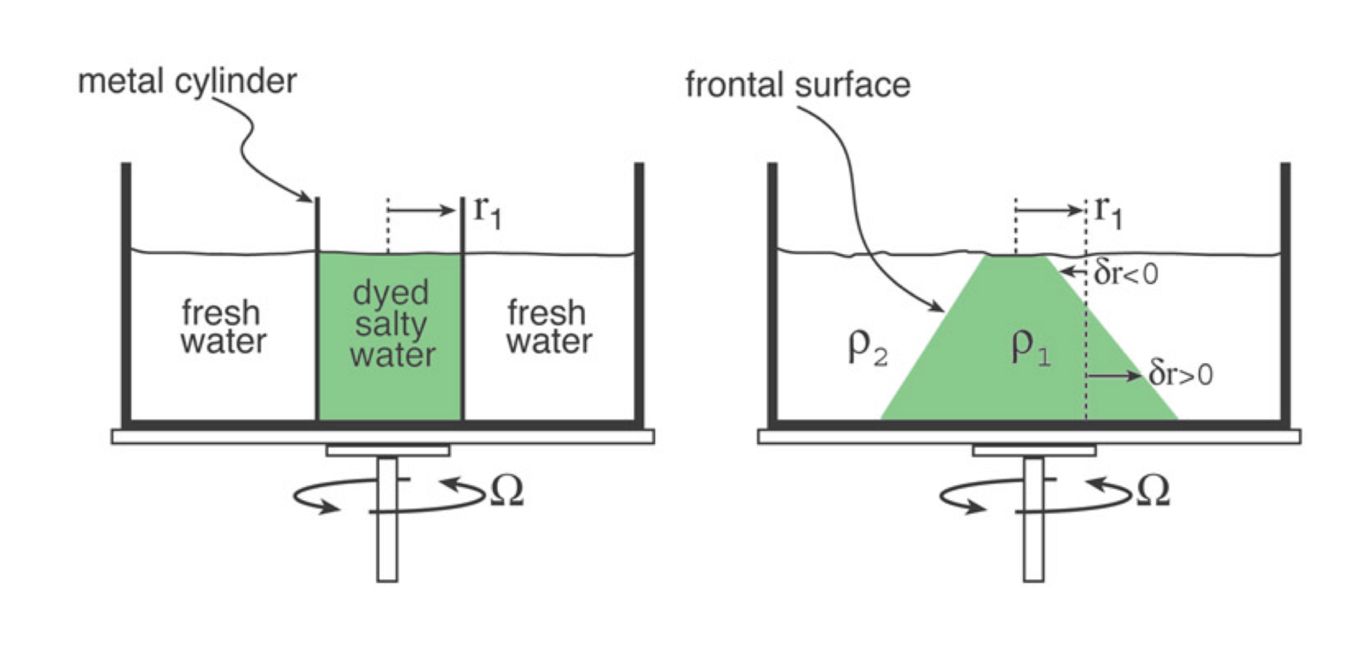
Figure 4.2: After the can is removed from the tank, the bottom of the dense fluid moves outwards, forming a cone. The less dense fluid converges towards the center of the tank, spiraling cyclonically in order to preserve angular momentum. The dense fluid spreads outwards, spiraling anti-cyclonically in order to preserve its angular momentum.2

Initially, the shape of the front resembles a Gaussian, with a wide sloping surface and flat top. As the experiment progresses, the frontal boundary gradually sinks relative to the free surface. Its sides flatten and the width of the center peak narrows (see Figure 4.2).

Using the equation for the deformation radius, given in 3.3, we calculate the predicted radius of deformation to be around 20 centimeters, or half of the width of the tank. Since the boundary of the front extends all the way to the outside of the tank, about 3/4 of the distance to the bottom of the tank, the actual radius of deformation for this front is slightly larger than this prediction. Therefore, we see the frontal boundary is horizontal towards the edge of the tank, as it has no more room to spread outwards.

Using the tracked particles, we now analyze the velocity of the fluid both on the surface and at the frontal boundary starting around 11 minutes after the removal of the can. As can be seen from the above images, the fluid appears sufficiently stable at this point in the experiment to assume hydrostatic balance. At this time, we track particles at the surface, resulting in the following set of tracks:

.

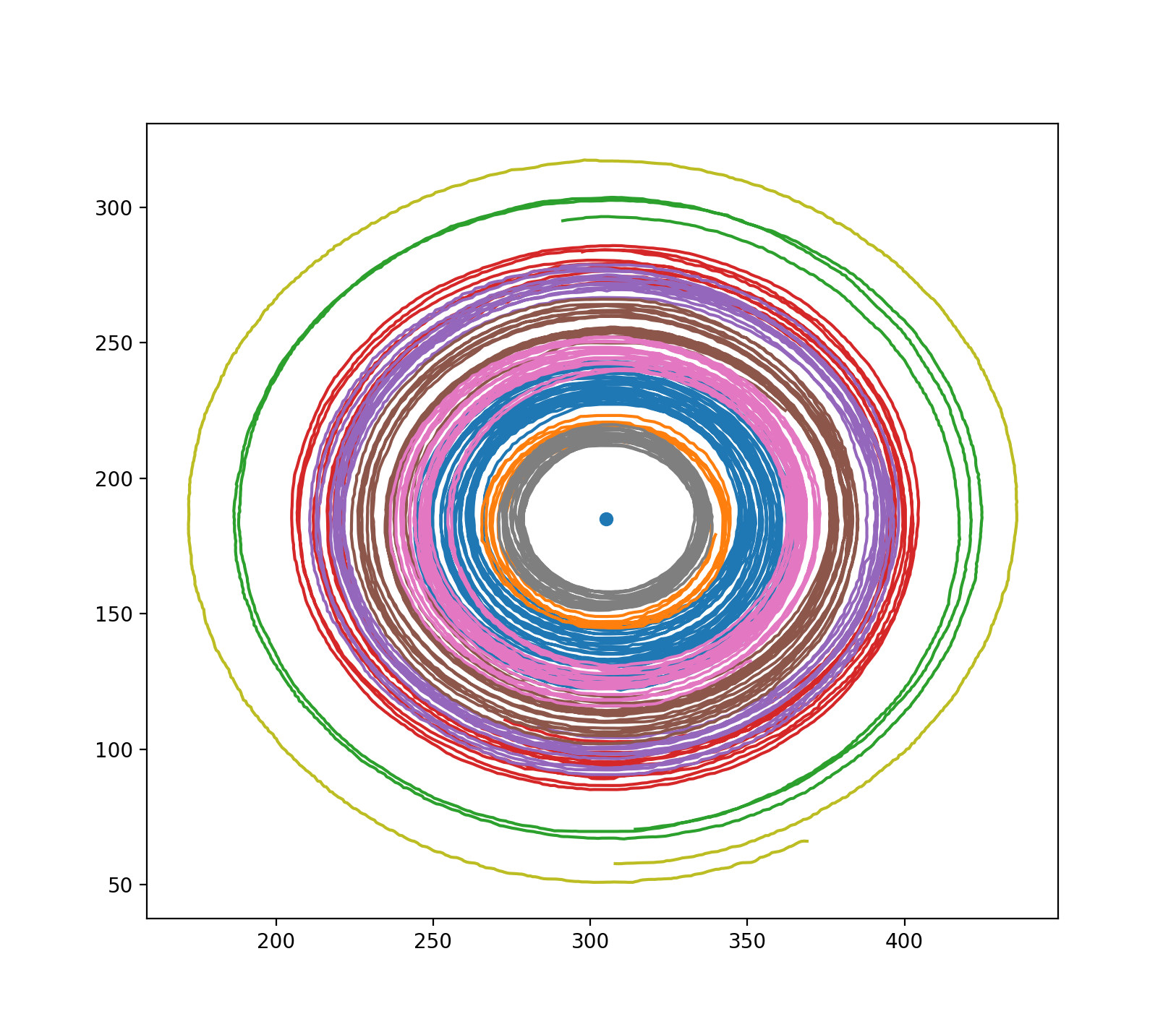
Figure 4.3: Trajectory of particles at the surface of the fluid tracked ≈11 minutes into the experiment, for ≈1 minute each. The axes are labeled in pixels, and the dot at the center indicates the center of the front. Each of the different colors corresponds to an individual tracked particle. The particles have small but noticeable radial displacement towards the center of the front.

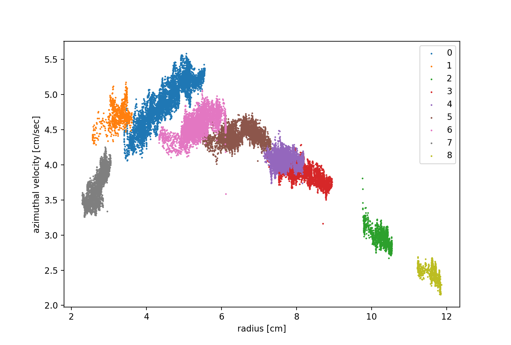
Figure 4.4: azimuthal velocity as a function of radius for the tracks shown in the Figure 4.2.

From the two above plots, one can see that the fluid does behave cyclonically at the surface, as we expected. At large radii, where the frontal boundary has a very small slope, the azimuthal velocity is small, as would be expected from the Margules relation. Notice that the maximum radius of the tracks is less than 12cm, whereas the edge of the tank is ≈20cm from the center of the front. At larger radii, the azimuthal velocity is nearly zero as the frontal slope is so small.

As the radius decreases, the slope increases and so does the azimuthal velocity of the fluid, reaching its peak at around 5cm. This radius approximately corresponds to the location of the edge of the can before it was removed. We would expect the pressure gradient at this radius to be largest, which implies fluid at this radius should also have the largest velocity (see equation 3.2). At small radii, the azimuthal velocity decreases again as the frontal boundary flattens and the pressure gradient decreases.

We also track the particles which sit just above the frontal surface. These are the blue spheres seen in Figure 4.1.

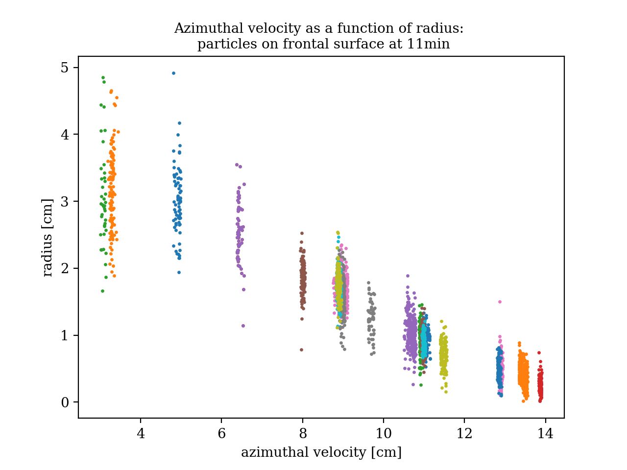
Figure 4.5: azimuthal velocity as a function of radius for particles tracked at the frontal boundary.

These particles are more difficult to track, hence the tracks are shorter, and the concentration of dye and particles at the center of the front makes it impossible to track the particles for very small radii accurately. Still, it is clear from this plot that the azimuthal velocity of the fluid at the frontal boundary has the same overall radial dependence as that of the fluid at the free surface for large radii. However, we see only a small peak at 5cm, unlike the very defined peak at that radius for the velocity of the fluid at the surface.

As expected, for the same radius, these particles have smaller azimuthal velocity than those at the surface. Upon removal of the can, the fluid at the surface is displaced towards the center more than the fluid at lower depths, therefore in order to preserve angular momentum the fluid at the surface must acquire greater azimuthal velocity (see Figure 4.2).

Using the Margules relation and the data collected for the velocity of particles at the boundary of the front to solve for the frontal slope, we "backed out" what the boundary of the front would look like according to the theory.

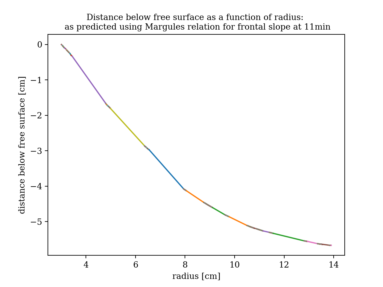
Figure 4.6: Predicted frontal boundary using the Margules relation at the velocity of particles tracked at the boundary. The particle with smallest radius was assumed to be near enough to the highest point of the frontal boundary. The largest radius of the tracked particles is about halfway between the center of the front and the edge of the tank.

Accurately comparing the images taken (Figure 4.1) to the plot above would be difficult due to issues of distortion. However, just looking at the 3rd image in Figure 4.1, the closest in time to when the particles were tracked, one can see that the overall shape of the front aligns well with the prediction. Therefore, we conclude that the Margules relation provides a good estimate for the shape of a front, given that the assumption of geostrophic flow holds.

5 Challenge: Inverting the Dome!

We were able to fairly successfully model a front formed after the collapse of a central denser fluid; naturally, we wanted to see if we could make the exact reverse scenario work. On our first iteration, we followed an identical procedure as in the regular dome version, but first put fresh water inside the cylinder, and filled the rest of the tank with salty water. We once again spun the tank up to 8rpm, removed the cylinder, aaaaaaand.............

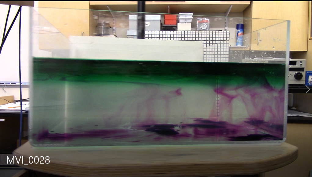
The front collapsed pretty much immediately. We added in some permanganate in a last-ditch effort to see something cool. You can judge for yourself whether this counts.

So, take 2. We figured our density difference was way too high - $\begin{array}{l}\frac{\Delta \rho}{\rho_{1}}\end{array}$ ~ 0.11! -and rotation rate too low (8rpm), such that the effects of gravity were much more influential than the effects of rotation. So, back to the drawing board.

This time, we decreased $\begin{array}{l}\Delta \rho\end{array}$ by a ton, making the salty water 0.96g/mL, only 0.02g/mL higher than the fresh water. We also kicked the rotation speed way up, to almost 21rpm. This time?

First problem: our camera was set to autofocus. Lesson learned.

Second problem: the front split up into many micro-fronts! We'd kicked omega up so high that the deformation radius. Eq.(3.3), was tiny. But this time, we could definitely see some inverted domes. Just, not well enough to get any slope readings.

So, try number 3. This time, we decided to do some math. We knew we wanted a deformation radius roughly on the order of the tank radius (or a bit smaller), and wanted to maximize the slope under that constraint. Fiddling around with Eqs. (3.2) and (3.3), we finally settled on $\begin{array}{l}\Delta \rho\end{array}$ ~ 0.25 g/mL, and a rotation rate around 9.5rpm. This time, things actually turned out...okay?

We definitely had fewer distinct peaks (and one very dominant peak), and they lasted for longer. But they still never quite stabilized, and we weren't able to pick out any slopes to test the Margules relation. It would probably take a lot more trial and error to find the right combination of $\begin{array}{l}\Delta \rho\end{array}$ and $\begin{array}{l}\Omega\end{array}$ to get a front that lasted, was distinct, and also didn't split. Even with the right parameters, chance, statistical variation, and the susceptibility of the phenomenon to hitting the edge of the tank and break apart, would make it tough to get this one consistently right.

6 Polar Atmospheric Front

The temperature of the air in the atmosphere does not gradually warm from the poles to the equator, but instead there is a sharp gradient between the cold air at the poles and the warmer air just south. As warmer air is less dense than cold air, the meeting of warm and cold air in the atmosphere produces a density interface like that seen in the lab. The whole system is rotating with the Earth, causing the formation of fronts.

.

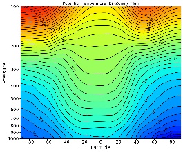
Figure 6.1: Left: Air temperature at 500mb for the Northern hemisphere in January. The change in temperature between the cold air at the North pole and the warmer air near the equator occurs only in the midlatitudes; otherwise, there is little meridional temperature gradient. This is because of the same phenomenon driving what we saw in the lab. Right: Potential air temperature as a function of pressure and latitude. Potential temperature is preserved under adiabatic processes and is therefore a better indicator of heat transport than temperature. Between 20 and 60 degrees latitude, there is a sharp potential temperature gradient where the polar front and warm air from southern latitudes meet at a positive slope relative to the poles.3

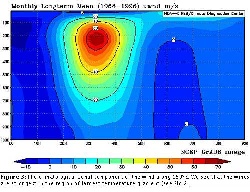
Figure 6.2: Wind speed as a function of pressure and latitude. Where the temperature gradient is largest, the wind speeds are also greatest. At around 60 degrees latitude, this temperature gradient produces the polar jet stream, which consists of powerful westerly winds. Just as in the lab, the boundary of the dense air in the polar cell forms a sloped boundary with the less dense, warmer air from the extratropics. 3

The gif above shows isosurfaces of the polar front, colored by wind speed. The winds at the surface form many small nonaxsymmetric fronts, similar to what we saw in our "reversed front" experiment. The higher altitude winds - the polar jet stream - create a full cyclonic circulation with the rotation of the Earth.

7 Polar Oceanic Front

In the ocean, ice melting from the poles brings light freshwater into contact with dense saltwater. Hence, Earth's rotation causes oceanic fronts to form, creating an anticyclonic circulation near the surface.

.

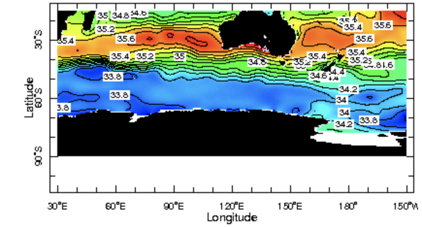
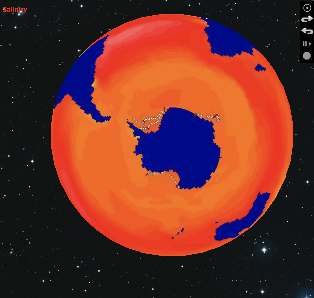
Figure 7.1: Left: salinity as a function of latitude. 4 Right: Four particles tracked off the coast of Antarctica on a time scale of 1.5 years. The particles move anti-cyclonically around Antarctica, largely due to the front that forms when the freshwater from the ice melting off Antarctica meets the salty, dense ocean water.

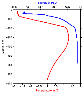
Figure 7.2: Salinity as a function of depth. Near the surface the water is cold and fresh, having melted from the ice on the poles. Between 100-200 meters deep the water becomes much saltier (and more dense), as well as warmer. There is a sharp gradient between the fresh and salt water; the boundary is known as a halocline. 5