...
To better understand Hadley circulation, a tank experiment was set up to mimic these atmospheric conditions in a controlled environment. A metal container filled with ice was placed in the center of a slowly rotating circular tank. The low rotation rate, 1.28 RPM, and correspondingly low Rossby number (f = 2Ω) was chosen to replicate the low latitude regions where the Hadley Cell forms. Five thermometers (labelled A through E) were placed on the outside of the ice bucket and along the sides and bottom of the plastic tank, in order to measure the generated temperature gradient.

Surface Flow:
Particle tracking software was used to track the motion of paper dots on the surface of the water, in order to determine how velocity varied as a function of distance. The tracks of the five particles studied, along with the plot of their velocities (in meters per millisecond) as a function of distance from the center of the tank, are included below. These surface flows in the tank correspond to the trade winds on Earth.

...
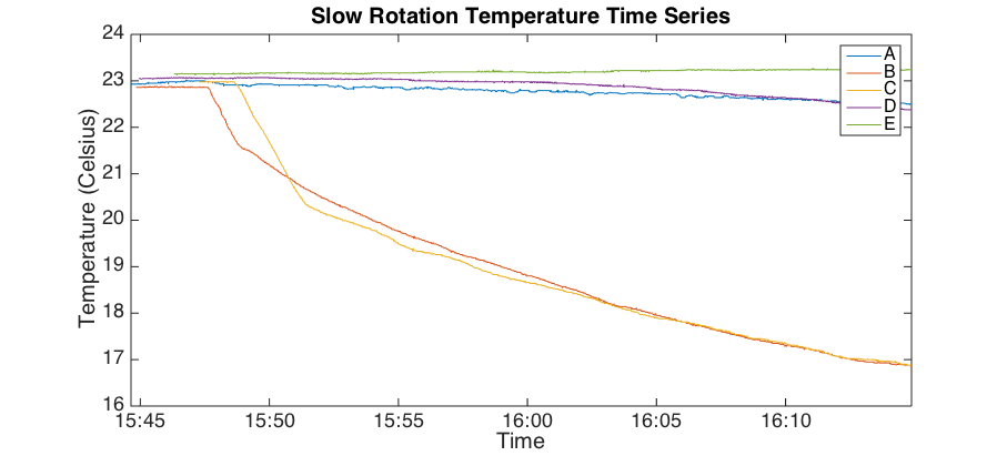
Thermometers B (at the bottom of the outer wall of the ice bucket) and C (on the bottom of the tank) clearly measure much colder temperatures than sensors placed elsewhere. The maximum temperature gradient recorded between B and D, both near the bottom of the tank, is roughly 5.5K The maximum gradient found at the top of the tank is .5K. Averaging these gives an approximate temperature gradient of 3K over the 18 cm region, or 16.67 K/m.
We can recall the thermal wind equation for an incompressible fluid that we derived in our study of fronts:...
We next plotted the zonally averaged meridional winds where positive values correspond to northward moving winds:

In the January plot, high altitude winds move toward the North Pole from the equator to around 30ºN and low altitude winds move from 30ºN to the equator. The opposite pattern is observed in July.
...

...
We can notice a couple interesting things from these plots. In the January when the Northern Hemisphere is experiencing winter, we see two clear maximums of Northward heat flux. These could be because the temperature gradient is strongest during the winter. The maximums are located on coasts where there are strong land-sea interactions. The combination of the stronger gradient and land-sea interaction could result in more synoptic scale storms and more eddies, resulting in stronger heat flux in those regions. In July when the Northern Hemisphere is experiencing summer, we observe that the northward heat flux is stronger overall in the Northern Hemisphere as well as more uniform. In both January and July, we see strong southward heat flux in the Southern Hemisphere.
...