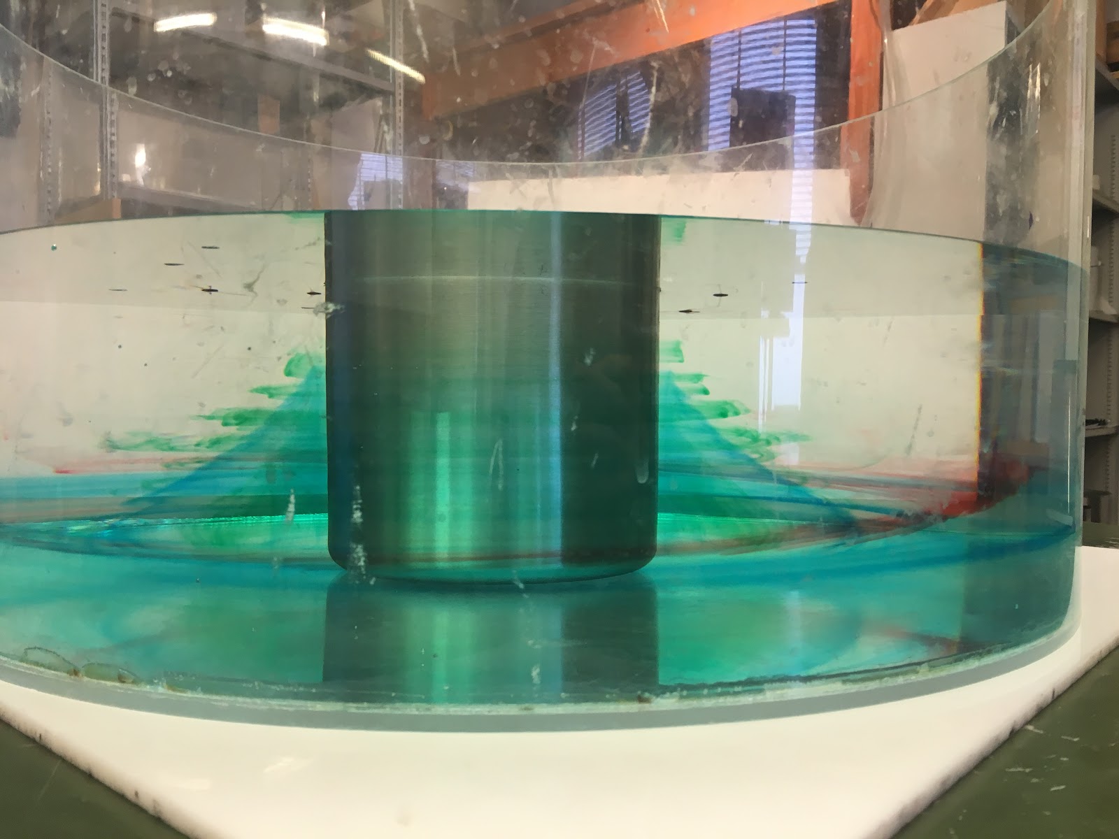
Versions Compared

Key

  • This line was added.
  • This line was removed.
  • Formatting was changed.

...

Section
borderfalse

Hadley

At low latitudes near the equator, atmospheric circulation is mostly axisymmetric. Warm air rises at the equator, moves to about 30ºN or south, where it then descends and returns to the equator. This circulation is called the Hadley Cell, which we will explore in more detail in this section.

Column
width50%

Tank Experiment

In order to imitate the circulation in the low latitudes, the first experiment was performed with a very slowly rotating tank - moving at just 1 revolution per minute. Observed from the counter-clockwise rotating reference frame, particles on the surface circled the tank, moving faster than the speed of the tank's rotation. Those towards the center of the tank were much faster than those on the outside. Dye dropped into the tank created trails that also circled the ice bucket. The dye that sank further moved more slowly and moved slightly radially outwards, while the dye that remained near the surface circled more quickly, and also moved radially inwards. These motions created a lengthening tendril of dye, which, seen from above, appeared to spiral towards the ice bucket.

P1010848.JPG

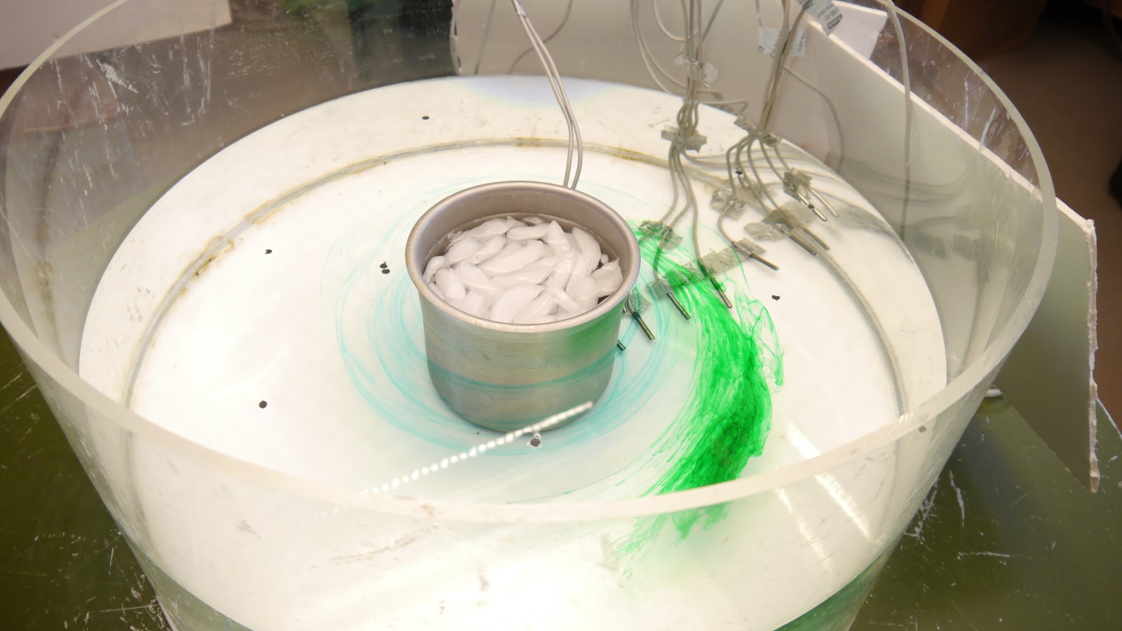
After many rotations, the spiral eventually morphed into a cone of dye around the ice bucket, just like the cone we saw in the second lab experiment. Potassium permanganate (bright purple streaks below) dropped onto the bottom of the tank also revealed the flows at depth. The dye created streaks that spread radially outwards and clockwise (counter the direction of rotation).

lowO.PNG

 Photo Apr 25, 2 05 48 PM.jpg

This behavior can be explained by radial overturning and thermal wind balance.

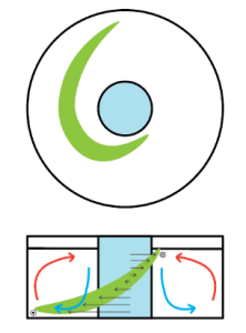
The cold water near the tank is more dense than the warmer water at the extremities, and hence sinks and spreads along the bottom due to hydrostatic balance:

hydrostatic balance.PNG

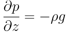
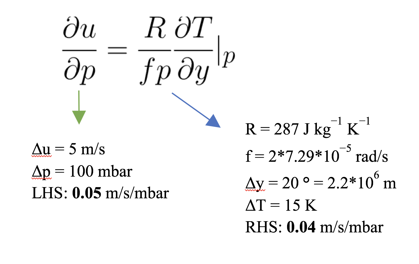
This states that the vertical pressure gradient is equal to the negative of the density times the gravitational acceleration. The result of this is that the dye at the surface moved inwards, and that at the bottom moved outwards.

However, the radial temperature gradient also imposes vertical wind shear, according to the equation for thermal wind:

thermal wind (T).PNG

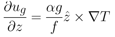
where the left hand side is the change in azimuthal velocity with height, α is the coefficient of thermal expansion, f is the coriolis parameter, and T is the temperature gradient. In the tank, the temperature gradient then causes "winds" to develop that increase in speed with height. This is why the dye spread into long trails around the ice bucket.

The positions of the particles at the surface could be monitored using a particle tracking software. Data showed that they followed circular paths around the center of the tank. Azimuthal velocities of the particles were calculated to be around 2 cm/s.

ptracks1-1.png


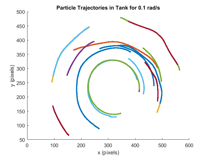
The temperature data from the thermometers revealed that an overall trend of decreasing temperature in the tank, as a result of the melting of the ice. The sensors at the bottom of the tank maintained a near-constant radial temperature over time, of about 4ºC. The temperatures higher up in the tank evolved differently however. The sensor on the edge of the tank measured a high temperature of about 21.2 ºC throughout the experiment, and the one on the ice bucket, gave a reading higher than all but the furthest sensor from the ice bucket at the bottom. These high temperatures are a result of the overturning circulation seen in the non-rotating case as well. Cold water near the ice bucket sinks and spreads along the bottom, leaving the surface water much warmer than that below.

tank T all.png

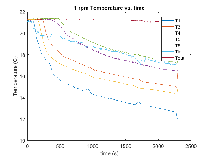
 Discretizing the equation for thermal wind and solving for u gives

u_geostrophic.PNG

where the coriolis parameter, f, has been replaced by 2Ω, L is the radial distance between the ice bucket and the edge of the tank, and H is the height of the water.

We can use the temperature data to calculate the right hand side of the equation, and compare it to the observed surface velocities of the paper dots.

hadley tank calc.PNG

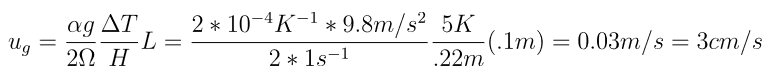
The result is close to the particle velocities found of about 2 cm/s, showing that the theory explains the observed phenomena well within margin of measurement and calculation error.


Column
width50%

Atmospheric Data

To draw a connection from the tank experiments to the real world phenomena, we investigated the selected month average from 1948 – 2017 atmospheric data including temperature, potential temperature, and wind speed at different locations and time around the earth.

For the Hadley regime, we found that the Meridional Wind, Omega, and Zonal Wind pattern in January differ from those in July.

Without considering the seasons, the is maximum solar heating region is near the equator since the region is almost perpendicular to the sun radiation. This orientation creates strong rising motion of the heating air.  The flow rises and diverges toward poles.  The direction now depends on the seasons. The hemisphere that experiences winter would have stronger temperature gradient; the flow tends to move toward that hemisphere. As the flow moves further from the equator, the air becomes closer to the Earth’s axis of rotation and starts experiencing more Coriolis forces. The zonal velocity must increase in order to conserve the momentum of the earth system; the maximum velocity is located around 30 degrees away from the equator where the subtropical jets located. Again, to determine the location of the the maximum, we need to know the time of the year; the hemisphere that experiencing winter would have the strongest zonal wind. Note that the zonal wind goes from west to east near the surface and east to west high up because of the rotation of the earth.  Because of the meridoonal wind, the air that just rises would go either in the north-south or south-north direction and go in the opposite direction once it sinks. Therefore, when the air sinks back to the surface, it moves in the opposite direction and closes the cell—fully completed Hadley Cells.

To elaborate a little bit more about the meridonal wind, we have to consider the horizontal temperature gradient at different latitude. We found that, as the wind moves further from the equator, it becomes colder near the surface, but it is opposite in the region high up above the Troposphere. 


.  The schematic that was described earlier is captured by the figures below.

To verify the relationship between the temperature gradient and the winds (thermal wind relationship), we overlaid the figures. We found that the most abrupt temperature change regions match the edges of the Hadley cells derived from the wind data.


To verify the relationship mathematically, we plugged the values from the plot to the thermal wind equations as the following.


Aim for the 500 mmb data, we can find the approximate value by using the nearby data points.

P = 450 mmb,  Zonal Wind = m/s                           Lat                      Lat = -55, temp = -25 degree C

P = 650 mmb, Zonal Wind = m/s                            Lat s                       Lat = -35, temp = -10 degree C      


From the thermal wind equation verification, we found that both sides of the equation have the same magnitude of the results. Therefore, we can say that in both cases, the flows are in thermal wind balance.

In conclusion, Hadley cell is responsible to the heat transport in regions where the effects of rotation are small—near the equator. The Hadley cell moves warm air toward the poles and cooler the air when moving it toward the equator. The strong Hadley cell can be determined by the hemisphere experiencing winter. Additionally, Hadley cell is also in thermal wind balance.


...