- Introduction
Due to differential heating and conservation of energy, as well as the Earth’s rotation and conservation of momentum, there is a general trend of energy and momentum transportation from the equator to the poles. The transport of heat from the equator to the poles is not done through just one large circulation from the equator the poles, but rather a couple smaller circulations limited in size by the effects of the rotation of the Earth. More specifically, due to the rotation of the Earth, the general circulation in the atmosphere breaks down into two main regimes:

1) the Hadley Cell transporting heat from the equator to midlatitudes
2) Eddies transporting heat from the midlatitudes to the poles
In this study, through the use of rotating tank experiments and analysis of atmospheric data, we examined the dynamics and energy transport involved in both the Hadley Cell and midlatitude eddies to study the general circulation of the atmosphere.
2. Hadley Circulation
2.1) Introduction:
Hadley circulation works to transport heat from the warm equator to midlatitudes. The Hadley Cell consists of warm air rising from the equator and moving poleward to 30ºN and 30ºS where it falls to the surface. Due to the Coriolis effect which turns winds to the right in the Northern Hemisphere and to the left in the Southern Hemisphere, this air moves westward at the equator and eastward in the midlatitudes around 30ºN and 30ºS.
2.2) Tank Experiment:
To better understand Hadley circulation, a tank experiment was set up to mimic these atmospheric conditions in a controlled environment. A metal container filled with ice was placed in the center of a slowly rotating circular tank. The low rotation rate, 1.28 RPM, and correspondingly low Rossby number (f = 2Ω) was chosen to replicate the low latitude regions where the Hadley Cell forms. Five thermometers (labelled A through E) were placed on the outside of the ice bucket and along the sides and bottom of the plastic tank, in order to measure the generated temperature gradient.

Particle tracking software was used to track the motion of paper dots on the surface of the water, in order to determine how velocity varied as a function of distance. The tracks of the five particles studied, along with the plot of their velocities (in meters per millisecond) as a function of distance from the center of the tank, are included below.


In addition to the motion of air towards and away from the equator, the Hadley circulation is also responsible for the trade winds, which travel along lines of roughly constant latitude. These trade winds are represented by the green dye, which was observed to spiral around the center of the tank. This spiral was also observed to form a sloping temperature surface, similar to the conical shape of the sloping density surface observed in the fronts experiment. While the frontal slope created in that experiment was due to the density difference between fresh and salty water, here the slope marked the colder, denser water, which had sunk to the bottom, and the warmer water on top.
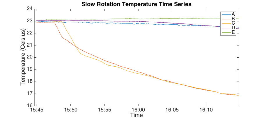
Thermometers B (at the bottom of the outer wall of the ice bucket) and C (on the bottom of the tank) clearly measure much colder temperatures than sensors placed elsewhere. The maximum temperature gradient recorded between B and D, both near the bottom of the tank, is roughly 5.5K The maximum gradient found at the top of the tank is .5K. Averaging these gives an approximate temperature gradient of 3K over the 18 cm region, or 16.67 K/m.
We can recall the thermal wind equation for an incompressible fluid that we derived in our study of fronts: