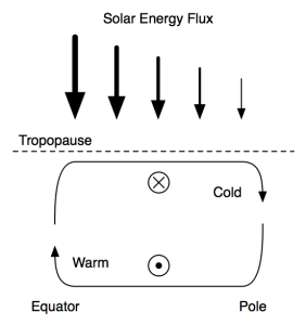
The Earth is not flat; different places receive different levels of insolation, leading to differential heating of the Earth's spherical surface. Due to the difference in the insolation received at the equator and that received at the poles, the additional energy received at the equator will rise and move towards the poles in order to balance the energy of insolation throughout the Earth's atmosphere. Likewise, cold air at the poles will sink and move towards the equator to complete the loop and satisfy continuity constraints on the flow of air in the atmosphere.
In a non-rotating environment, this movement is straightforward; a simple cycle of air from the cold poles to the warm equator and back would form. This movement is complicated in practice by the rotation of the Earth. As the air at the equator moves toward the poles, its distance from the Earth's axis of rotation decreases and the conservation of its rotational momentum will cause the northward-moving air to curve to the right according to the Coriolis force. Likewise, the air moving back towards the equator will also curve right. This circular motion of air is known as a Hadley cell.
The Trade Winds
On Earth, this Coriolis-forced wind movement results in the phenomenon known as the trade winds. Above about the 30th parallel, the conservation of momentum causes a breakdown in the regime of the Hadley cell, and air sinks. It is possible to observe this in practice by first studying the potential temperature, θ, averaged over all longitudes.
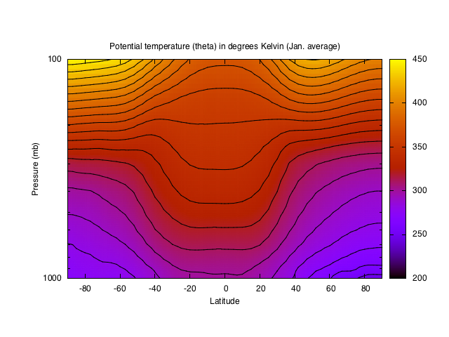
This plot, which depicts the average potential temperature in the atmosphere in January demonstrates the warmer temperature observed near the equator, and colder temperatures observed near the poles. The center of the warmer temperatures appears to the south of the equator, due to the southern position of the sun in January. Likewise, cooler temperatures are observed over the North Pole rather than the South Pole. What is particularly notable about this plot is that the potential temperature is actually cooler in the stratosphere over the tropics than it is over the poles, indicating that the higher altitudes are warmed over the poles, where the lower altitudes are warmed near the surface. The gradient of the potential temperature is clearly visible over the mid-latitudes, but is essentially non-existent over the tropics, indicating thorough mixing of the air in the tropical region in which the Hadley cell dominates.
The warm temperature over the tropics translates to rising motion, which may be determined from the average value of ω, the vertical movement of the air, as averaged over all longitudes.
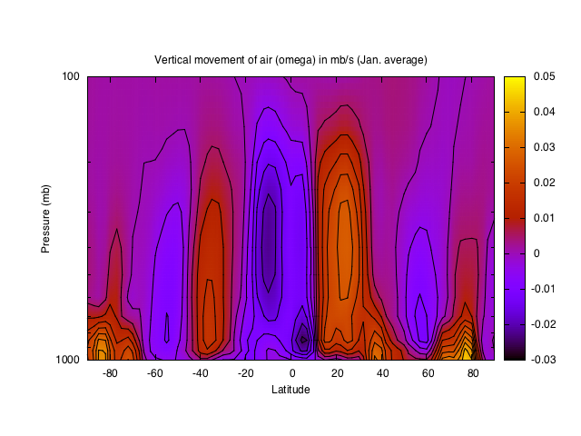
Here, air may be observed to rise close to the equator and sink near 25 degrees north latitude. Since this average is the January average, during winter in the northern hemisphere, the strongest movement is observed in the northern hemisphere, where the temperature gradient is strongest. Similarly, the sinking motion is observed at a lower latitude due to the axis pointing away from the sun. The meridianal movement of the air may also be plotted to demonstrate that this rising and sinking is connected in a single cell.
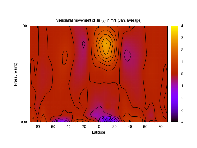
The Hadley cell is visibly completed by the stronger southerly movement of about 3 m/s near the top of the rising column at about the 150mb level, and stronger northerly movement near the surface. The latter movement is the meridianal component of the trade winds. The zonal component may also be plotted to demonstrate the effects of the Coriolis force on the northerly winds at the surface.
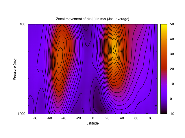
Easterly winds are clearly evident at the surface, ranging up to nearly 10 m/s about the 900 mb level. The westerly winds aloft are less visible, due to the dominant westerly flow of the jet stream north of the 30th parallel. Even so, a slight extension of weak westerly winds may be observed to extend down nearly to the equator, which is suggestive of the westerly contribution of the top part of the Hadley cell.
Tank
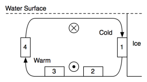
It is possible to visualize the movement of the Hadley cell in a rotating tank of water to verify the expected "winding" and "unwinding" of the Hadley cell. A temperature gradient may be created in a slowly rotating tank of water (< 1 rpm) by placing a container of ice in the middle of a rotating tank of water. Water will then cool next to the tank, sinking and slowly flowing outwards. Continuity will then ensure that warm water on the outside of the tank will flow inward to replace the cool, sinking water. As it moves inward, the warmer surface water should move in the direction of the rotation of the tank of water.
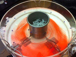
I performed this experiment with my partner Phoebe Henderson, in which we placed two sets of four thermistors, one on the center ice canister (1), one on the outer rim of the tank (4), and two on the bottom of the tank, one placed 2–3cm from the side of the canister (2), and the other 10–11cm from the canister (3). The tank was spun at 0.95 rpm (one revolution ever 62 seconds) and allowed to reach a steady state before ice was added. Paper dots were then tracked to determine the shear in the Hadley cell. Finally, dye was dropped into the tank to observe the shear in detail.
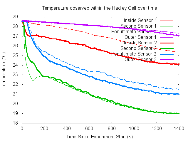
The evolution of the temperature observed at each sensor over time may be plotted.
Analysis of the Tank Experiment
What is perhaps the most fascinating finding from this plot is how the innermost sensor on the can is much warmer than either of the two sensors on the bottom. This stands to reason, however; as the warm water on the surface reaches the canister containing the ice, it only begins to cool. It only reaches its maximum coolness at the bottom of the cylinder, at which point it flows outward to reach the "second" and subsequently the "penultimate" sensor. As a result, the "second" sensor is the coolest, and the "penultimate" sensor appears second coolest. The outermost sensor barely cools at all, outside of the cooling due to radiation out of the tank.
Another notable pattern in the data is the periodic variation in the temperature observed at most sensors. This might be a result of an off-center alignment of the tank. This would create an imbalance and seiching of the water in the tank. As a result, each sensor would periodically move through warmer and colder water having the same period as the rotation, which this variation appears to have.
It is possible to numerically verify the shear created by the Hadley cell by applying the thermal "wind" equation for water which varies in temperature,

Where α is the thermal coefficient of expansion of water and Ω is the rotation rate of the tank. By taking the temperature difference between the two bottom sensors (approximately 2K over 8cm), we may obtain a value for ΔT, which may be substituted into the thermal wind equation to calculate the expected shear, 2.45 m/s per meter. As the depth of the water in the tank was 9 cm, the speed of the rotation of the dots observed on the top of the water would be expected to be approximately 0.22 m/s.
Several particles were tracked on the surface of the tank. These tracks can be used to plot the azimuthal velocity of the dots relative to the distance from the center of rotation (as averaged over a one second period around a given point in time).
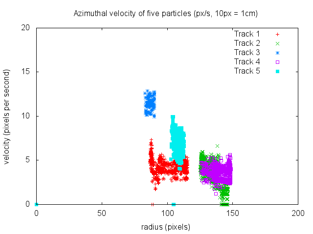
What is surprising about this plot is the order of magnitude difference of the observed velocities (about 0.5–1 cm/s) and the expected velocity of 22 cm/s. Although we did not measure temperatures throughout the water column, the difference of the bottom temperatures from the side-temperatures suggests that the cool temperatures are only observable in a thin layer very close to the bottom of the water column. Assuming a perfect adherence to the thermal wind equation, the height of the cool water would then be only 4 mm.