Acceleration
The time rate of change of velocity.
MathematicalRepresentation"> Mathematical Representation
One-DimensionalAcceleration"> One-Dimensional Acceleration
UtilityoftheOne-DimensionalCase"> Utility of the One-Dimensional Case
As with all vector equations, the equations of kinematics are usually approached by separation into components. In this fashion, the equations become three simultaneous one-dimensional equations. Thus, the consideration of motion in one dimension with acceleration can be generalized to the three-dimensional case.
GraphicalRepresentationsofAcceleration"> Graphical Representations of Acceleration
The one-dimensional form of the definition of acceleration:
\begin
[ a = \frac
] \end
indicates that acceleration is the slope of a velocity versus time graph.
Since velocity is the derivative of position:
\begin
[ v = \frac
]\end
we can also write:
\begin
[ a = \frac{d^
x}{dt^{2}}]\end
Thus, we can also see the effects of acceleration in a position versus time graph like that shown here:

Consider the position vs. time graph shown above. If you were to lay a ruler along the curve of the graph at the origin, the ruler would have to be horizontal to follow the curve, indicating zero slope. Thus, the velocity is zero at the origin. As you follow the curve, however, the ruler would have to be held at a steeper and steeper angle (see the lines added in the graph below). The slope grows with time, indicating that the velocity is becoming more and more positive (the speed is increasing). This positive change in velocity indicates a positive acceleration. In calculus terminology, we would say that a graph which is "concave up" or has positive curvature indicates a positive acceleration.

Examples that use the graphical representations of acceleration are:
TheDangerofDeceleration"> The Danger of Deceleration
Acceleration poses a problem for the specialized vocabulary of physics. The other two major kinematical quantities, velocity and position, have a related scalar quantity. For instance, distance is a scalar that is related to displacement. Speed is a scalar that is related to velocity. If we are discussing instantaneous velocity, then speed is the magnitude of velocity. The acceleration can also be discussed in terms of a vector acceleration or simply the magnitude, but for acceleration we have no special term for the magnitude. The vector is called "the acceleration" and the magnitude is "the magnitude of the acceleration". This can result in confusion.
This problem is exacerbated by the fact that in everyday language, we often discuss distance, speed and acceleration. The everyday definitions of distance and speed are basically equivalent to their physics definitions, since we rarely discuss direction of travel in everyday speech and these quantities are scalars in physics (no direction). Unfortunately, in physics, we usually use the term "acceleration" to refer to a vector, while in everyday speech it denotes a magnitude.
The difficulties do not end there. Everyday usage does make one concession to the vector nature of motion. When we discuss acceleration in everyday speech, we usually specify whether the object is "accelerating" (speeding up) or "decelerating" (slowing down). Both terms imply a change in velocity, and so in physics we can call either case "accelerating". The physics way of explaining the difference is:
everyday term |
physics equivalent |
|---|---|
acceleration |
acceleration and velocity point in the same direction |
deceleration |
acceleration points in the direction opposite the velocity |
To understand the physics definition, imagine a child on a playground swing. If you want to help the child swing faster, you must push them in the same direction as they are currently moving (so the acceleration of your push is in the same direction as the child's velocity). If you want to help them slow down, you must push them in the direction opposite their current motion (so that the acceleration of the push points opposite to the velocity).
The difference between acceleration and deceleration (in the everyday sense) can also be illustrated graphically:
positive acceleration |
negative acceleration |
negative acceleration |
positive acceleration |
|---|---|---|---|
|
|
|
|


Both the graphs that show "acceleration" have slopes that are steepening with time. The only difference is that one of the graphs has a steepening positive slope and the other has a steepening _negative slope. Both graphs showing "deceleration" have slopes that are approaching zero as time evolves. (Again, one has a negative slope and one has a positive slope.)
It is a very common misconception that a negative acceleration always slows down the object it acts upon. This is not true. It is important to note that a graph which has a negative slope approaching zero (slowing down) implies a positive acceleration, and a graph which has a negative slope that is steepening (speeding up) implies a negative acceleration. It may help you to remember that the concavity of the graph specifies the direction of the acceleration.
ConstantAcceleration"> Constant Acceleration
Integration with Respect to Time "> Integration with Respect to Time
If acceleration is constant, the definition of acceleration can be integrated:
\begin
[ \int_{v_{\rm i}}^
dv = \int_{t_{\rm i}}^
a\: dt ] \end
For the special case of constant acceleration, the integral yields:
\begin
[ v - v_
= a(t-t_
) ] \end
which is equivalent to:
\begin
[ v = v_
+ a (t-t_
) ] \end
We can now substitute into this equation the definition of velocity,
\begin
[ v = \frac
]\end
which gives:
\begin
[ \frac
= v_
+ a t - a t_
] \end
We can now integrate again:
\begin
[ \int_{x_{\rm i}}^
dx = \int_{t_{\rm i}}^
\left( v_
- at_
+ a t\right)\:dt ] \end
to find:
\begin
[ x - x_
= v_
(t-t_
) - a t_
(t-t_
) + \frac
a( t^
- t_
^
) ] \end
We finish up with some algebra:
\begin
[ x = x_
+ v_
(t-t_
) + \frac
a (t^
- 2 t t_
+ t_
^
) ] \end
which is equivalent to:
\begin
[ x = x_
+ v_
(t-t_
) + \frac
a (t - t_
)^
] \end
Integration with Respect to Position "> Integration with Respect to Position
The definition of acceleration can also be integrated with respect to position, if we use a calculus trick that relies on the chain rule. Returning to the definition of acceleration:
\begin
[ \frac
= a ] \end
we would like to find an expression for v as a function of x instead of t. One way to achieve this is to use the chain rule to write:
\begin
[ \frac
\frac
= a ] \end
We can now elminate t from this expression by using the defnition of velocity to recognize that dx/dt = v. Thus:
\begin
[ \frac
v = a ] \end
which is easily integrated for the case of constant acceleration:
\begin
[ \int_{v_{\rm i}}^
v \:dv = \int_{x_{\rm i}}^
a \:dx ] \end
to give:
\begin
[ v^
= v_
^
+ 2 a (x-x_
) ] \end
One-DimensionalMotionwithConstantAcceleration"> One-Dimensional Motion with Constant Acceleration
Four or Five Useful Equations "> Four or Five Useful Equations
For a time interval during which the acceleration is constant, the instantaneous acceleration at any time will always be equal to the average acceleration. Thus, by analogy with the definition of average velocity, we can write:
\begin
[ a = \langle a\rangle_
= \frac
= \frac{v - v_{\rm i}}{t - t_{\rm i}} ] \end
Taking this equation as a starting point and using the relationship between average velocity and position
\begin
[ \langle v\rangle_
= \frac
= \frac{x - x_{\rm i}}{t- t_{\rm i}} ] \end
We removed the bar in the acceleration equation above because acceleration is constant. We cannot similarly drop the bar in the average velocity equation, because velocity is not constant when acceleration is constant, except in the special case that a = 0 (and in that case, you should really use the simpler model for constant velocity.
lets us derive five very important equations.
Three of these equations follow directly from the integrations performed in the section above.
\begin
[ x = x_
+ \bar
(t-t_
) ] [ \bar
= \frac
(v+v_
) ]
[ v = v_
+ a(t-t_
) ][ x = x_
+ v_
(t-t_
) + \frac
a (t-t_
)^
]
[ v^
= v_
^
+ 2 a (x-x_
) ]\end
Because the first equation is not specific to the case of constant acceleration (it is simply a definition of average velocity) it is combined with the second equation in the summary on the model specification page for one-dimensional motion with constant acceleration.
A Training Flight (Some Typical Exercises)"> A Training Flight (Some Typical Exercises)
|
Photo by Craig Kinzer, courtesy Wikipedia. |

The Piper Tomahawk, widely used for flying lessons, has a liftoff speed of about 55 knots and a landing speed of about 46 knots. The listed ground-roll for takeoff is 820 feet, and for landing is 635 feet.
Part A
Assuming constant acceleration, what is the Tomahawk's acceleration during the takeoff run?
Solution
System:
In each of the parts, we will treat the Tomahawk as a point particle.
Interactions:
We are assuming that the thrust from the plane's engine, air resistance, rolling friction, and all other influences add up to give a constant acceleration.
Model:
One-Dimensional Motion with Constant Acceleration.
Approach:

Part B
What is the elapsed time from the instant the plane begins its takeoff run until it lifts off the ground?
Solution
System, Interactions and Model: The system, interactions and model are the same as in Part A.
Approach:
Part C
How far does the plane travel in the first 9.0 seconds of the takeoff?
Solution
System, Interactions and Model: As in the previous parts.
Approach:
Part D
What is the acceleration during landing?
Solution
System, Interactions and Model: As in the previous parts.
Approach:

Part E
How far does the plane travel in the first 9.0 seconds of the landing?
Solution
System, Interactions and Model: As in previous parts.
Approach:
The Utility of Constant Acceleration"> The Utility of Constant Acceleration
Stringing together a series of constant velocity segments is not usually a realistic description of motion, because real objects cannot change their velocity in a discontinuous manner. This drawback does not apply to constant acceleration, however. Objects can have their acceleration changed almost instantaneously. For example, you could be coasting along in a car at a constant 60 mph with zero acceleration when suddenly you see traffic stopped ahead. If you slam on the brakes, your car will still be going 60 mph for an instant, then it will drop to 59, 58, 57, etc. Your acceleration, on the other hand, has almost instantly changed from zero to a substantial acceleration directed opposite your motion. You can feel this abrupt change as a passenger as you are forced against your seatbelt. Similarly, when an airplane begins its takeoff run, you can feel yourself suddenly pressed back in your seat as the plane's acceleration changes almost instantaneously from 0 to a significant forward acceleration. Because of this, it is often reasonable to approximate a complicated motion by separating it into segments of constant acceleration.
An Exercise in Continuity"> An Exercise in Continuity
Suppose an object is moving along a one-dimensional position axis. The object starts its motion at t = 0 at the position x = 0 and with velocity v = 0. It has an acceleration of +2.0 m/s2. After 4.0 seconds, the object's acceleration instantaneously changes to - 2.0 m/s2. Plot velocity and position versus time graphs for the first 8.0 seconds of the object's motion.
Solution
System:
The object will be treated as a point particle.
Interactions:
The accelerations as described in the problem.
Model:
One-Dimensional Motion with Constant Acceleration, applied twice to cope with the change in acceleration.
Approach:
Understand the Limitations of the Model
We will have to use the model twice. Even though the acceleration has a size of 2.0 m/s2 throughout the motion, the direction of the acceleration changes at t = 4.0 s. Therefore, the acceleration is not constant over the first 8 seconds of the motion. The acceleration is, however, separately constant in the time intervals from 0 to 4 seconds and from 4 to 8 seconds. We will therefore have to use the model twice: once to describe the motion from t = 0 seconds to t = 4.0 seconds, and once more to describe the motion from t = 4.0 seconds to t = 8.0 seconds.
The First Interval
For the first part of the motion, our givens are:

We begin by finding the velocity. The simplest Law of Change appropriate to our givens is:

which, after substituting the givens, tells us:

This is the equation for a line with slope 2 and intercept 0, giving the graph:

We then find the position. The most direct Law of Change is:

which yields the parabolic graph:

The Second Interval
We now wish to analyze the second part of the motion. In this part of the motion, we must change our givens. We now have ti = 4.0 s, t = 8.0 s, and a = – 2.0 m/s2. Unfortunately, this is not enough. We do not know xi, x, vi or v. We have too few givens to proceed.
The answer to this dilemma is simple. We have just derived expressions that give x and v for any time between 0 s and 4.0 s. We would like to know x and v at 4.0 s. Thus, we can use the final time of the first part of the problem to obtain the initial conditions for the second part. From our graphs or from the equations, we can complete our list of givens for the second part:

This allows us to write an equation for the velocity:

and the position:

Putting them Together
These new expressions can be used to finish the plots we started in the first part. Plotting the functions from the first part in the interval t = 0 s to t = 4.0 s and the functions from the second part in the interval t = 4.0 s to t = 8.0 s gives the complete graphs shown below. For completeness, we also show the acceleration graph.


Here we can see that although the acceleration is discontinuous (has a break in the graph at t = 4.0 s) the velocity is not discontinuous. The velocity is a connected graph, though it does display a kink at 4.0 s, when the graph suddenly takes a sharp bend. This kink is a sign of a discontinuous 1st derivative (the 1st derivative of velocity with respect to time is acceleration, which is discontinuous). The position, however, is completely smooth. It is connected and displays no kinks. (The first derivative of position is velocity, which is continuous.)
We ensured that the position graph would be smooth when we set the initial position and velocity of the second portion of the motion equal to the final position and velocity of the first portion!
The fact that smooth position curves are obtained from a motion composed of a sequence of motions with constant acceleration is a major reason that modeling a motion using segments of constant acceleration is a powerful tool.
Example Problem – Fan-Powered Ice Boat"> Example Problem – Fan-Powered Ice Boat

Pictured here is the University of Manitoba Center for Earth Observation Science's air/ice boat "Skippy" (photo courtesy CEOS). Skippy has a large fan at the back to allow it to accelerate as it slides across icy surfaces. Suppose you are piloting a similar craft on very slippery ice which will not slow the boat at all if it is coasting. Suppose also that the fan on your boat can be reversed instantanously, switching its direction of thrust from forward to backward. Assume the action of the fan (when it is on) always produces an acceleration with the same constant magnitude. Air resistance is negligible.
This simple model of the air/ice boat is not realistic. We have chosen it to illustrate the properties of motion with constant acceleration. As you work through this example, decide which aspects are contradicted by your own experience. How would you develop a more realistic model of the boat's behavior?

For the questions in this example, use the following coordinate system (illustrated above). You have a Base Camp at position x=0. Your assignment is to make observations of ice thickness and atmospheric conditions at two stations. Station One is 1 mile east of Base Camp, and Station Two is 2 miles west of Base Camp. Take east to be the positive x-direction.
Problem 1
Part A
Suppose you have left Base Camp and are halfway to Station One. You have been accelerating to the east the entire trip, but you now realize you have forgotten your gloves. You immediately flip the fan control switch to backward, reversing the direction of the thrust. Describe in words what will happen to your position and your velocity from the instant you reversed the fan.
Solution
System:
The boat and its contents will be treated as a point particle.
Interactions:
An external force from the action of the fan (actually from the air that the fan is pushing).
Model:
One-Dimensional Motion with Constant Acceleration
Approach:
Part B
Sketch rough graphs of your velocity and position as a function of time from the instant the fan was reversed.
Solution
System, Interactions and Model: As in Part A.
Approach:


Part C
Given that the boat was halfway to Station One before you reversed it, that it started from rest at Base Camp, and that the fan was accelerating the boat forward until the instant you reversed it, where will the boat be when it (instantaneously) comes to rest after you have reversed the fan?
System and Interactions: As in Part A.
Model:
To correctly answer this part, you will have to model the boat's motion starting from Base Camp. The model is still One-Dimensional Motion With Constant Acceleration, but it has to be applied twice. First, there is the eastward acceleration from the time that you leave Base Camp until you reverse the fan. Then, there is the westward acceleration model of Part A.
This technique of breaking up a complicated motion into more-easily-modeled pieces is both frequently used and extremely powerful.
Approach:

Part D
Suppose that once you have reversed the fan, you keep the fan reversed and on. Will you arrive safely back at Base Camp?
Solution
System, Interactions and Model: As in the previous parts.
Approach:
Problem 2
Suppose you are making your daily rounds. This involves:
- starting from rest at the Base Camp
- traveling to Station Two
- remaining at Station Two for the same amount of time it took to get there
- turning the boat around and traveling to Station One (without stopping at Base Camp)
- remaining at Station One for the same amount of time you were at Station Two
- turning the boat around and returning to Base Camp and stopping there
Part A
Sketch graphs of your position and velocity as a function of time for your entire daily rounds. Assume that whenever you travel, you accelerate toward the destination for exactly half the trip and then decelerate for the other half.
System, Interactions and Model: As in the previous problem.
Answer:

Part B
Divide your graphs into segments and label each segment with the position of the fan switch (forward, backward or off) during that segment. Remember that in your daily rounds, you always turn the boat before setting off from Base Camp or the Stations to point in the direction you are moving.
Solution
System, Interactions and Model: As in the previous problem.
Approach:


Problem 3 - Challenge
In Problem 2 we assumed that the best way to travel is to speed up for half the trip and then slow down for the second half. This gives your craft the greatest controllable speed (assuming you don't want to hit something at your destination to stop), but it also requires you to decelerate much earlier than if you just turned off the fan and coasted for a while at some intermediate speed. Assuming you want to minimize the time to your destination, what is the best way to use the fan?
Near-Earth Gravity"> Near-Earth Gravity
One of the most important applications of One-Dimensional Motion with Constant Acceleration is describing the motion of objects moving vertically under the influence of [gravity]. For objects near the surface of the earth, gravity creates a constant pull directed essentially straight toward the ground.
Because of the earth's enormous size, "near the surface" applies to anywhere that ordinary people will travel. In fact, even the space shuttle in orbit is experiencing an acceleration of around 8.7 m/s 2 (only 12% less than the acceleration of gravity at the surface of the earth) toward the earth's center. (The astronauts do not "feel" this acceleration for reasons to be discussed in a later lesson.)
Interestingly, the gravitational acceleration produced by the earth is not only constant on objects near its surface, but it is also exactly the same magnitude for all objects if air resistance is negligible. That value is:
\begin
[ g = 9.8\:
^
]\end
Air resistance is often non-negligible if 99% accuracy is desired. Neglecting air resistance is generally reasonable for ballpark (good to within 10%) estimates, provided that the object is not of an extremely low density (e.g. a beach ball), or of a shape that interacts with the air to produce lift (e.g. feathers, sheets of paper). The reasonableness of ignoring air resistance depends heavily on the distance of the fall. For example, it is an excellent approximation to ignore air resistance on a baseball dropped from a table, a reasonable ballpark estimate to ignore air resistance on a baseball thrown (hard) straight upward, and a terrible estimate to ignore air resistance on a baseball dropped from an airplane 2 miles above the ground.
Example Problem – Keys Please"> Example Problem – Keys Please
A college student with a third floor dorm room is exiting the dorm when he suddenly realizes he has forgotten his keys. Rather than run back to the room, he calls his roommate and goes to stand under the dorm room window. The roommate brings the keys to the window.
Part A
Suppose the roommate drops the keys straight down. The keys are released at rest from a height h= 5.0 m above the outstretched hand of the forgetful student. How long are the keys in the air from the time the roommate releases them until the instant they land in the student's hand?
Solution
System:
The keys will be treated as a point particle.
Interactions:
The earth has an influence on the keys, giving them a constant downward acceleration of magnitude g.
Model:
One-Dimensional Motion with Constant Acceleration. The keys are in freefall with a constant acceleration from gravity. We will choose our axis such that the positive direction is upward.
Approach:


Part B
Suppose that, instead of dropping the keys, the roommate tosses them straight up with an initial speed of 3.3 m/s. The keys are released from a height h= 5.0 m above the outstretched hand of the forgetful student. How long are the keys in the air from the time the roommate releases them until the instant they land in the student's hand?
Solution
System, Interactions and Model: The system, interactions and model are the same as for Part A.
Although the keys do receive an acceleration from the roommate while they are in contact with his hand, the instant they leave the roommate's hand gravity takes over. The observational evidence of this is that the keys will immediately begin to slow down, indicating the action of a downward force.
Approach:
We will illustrate two separate but completely equivalent ways to do this problem. The first way is faster, but requires familiarity with the quadratic equation. The second way avoids the quadratic equation by making use of symmetry, but it requires more physical insight.
With Quadratic
The problem is identical to Part 1 except that vi is not zero. Thus, the equation that we have to solve is:

This is a quadratic equation. It is a good idea to rearrange it:

so that it is clear that we have an equation of the form

if we choose:

Using these assignments in the quadratic equation gives:

To obtain a positive time, the positive sign must be chosen since the radical expression will clearly evaluate to be larger than vi, so:

The negative root is unphysical in this problem, since the keys were not in freefall until released at t=0. The negative root could have physical meaning in another problem, however, if the system was in freefall both before and after t = 0.
Without Quadratic
|

Freefall (and later, projectile) problems can often be usefully broken into two parts and analyzed in a mathematically straightforward fashion. The point at which we will separate the problem into two parts is the point of maximum height. As we will see, this is a useful choice because the velocity goes to zero at that point. We begin by analyzing the upward motion of the keys.
Considering only the trip up to maximum height (shown in blue in the figure at right), we know both the initial and final velocities. Since we also have the acceleration (gravity), this information allows us to use the simplest available Law of Change in our model:

so, using a=-g and v=0:

We have the time, which is what we wanted, but we must now make a slight detour and find how far the keys travel during their upward motion. The reason for this is that (as you will see) we will need that height to find the time the keys take to fall down from the peak to the student's hand. Luckily, this distance is easy to find. There are many equations that can be solved for it, but we will choose the one that is mathematically simplest:

Now if we use our expression for tup and the fact that v = 0 at the peak, we find that the distance traveled up from the roommate's hand is:

.
We are now ready to solve for the time to fall down from the peak (the part of the path shown in red in the figure at right). The solution proceeds exactly as in Part 1, so we use that result. The only change is that the keys are now falling from a total height of:

Then, using the answer to Part A, the time to fall is:

The total time is:

The same answer obtained using the quadratic formula.
Part C
As a final illustration, suppose that the roommate throws the keys downward with an initial speed of 3.3 m/s. The keys are released from a height h= 5.0 m above the outstretched hand of the forgetful student. How long are the keys in the air from the time the roommate releases them until the instant they land in the student's hand?
Solution
System, Interactions and Model: As in the previous parts.
Approach:
As in Part B, we will illustrate two separate but completely equivalent ways to do this problem. The first way is one step, but requires familiarity with the quadratic equation. The second way avoids the quadratic equation, but it requires two steps and stronger physical insight.
With Quadratic
The solution is exactly the same as for Part B. The only difference is that vi = -3.3 m/s instead of +3.3 m/s. Thus, we find:

Without Quadratic
This time, the motion has no peak point at which the keys are turning around. Thus, we cannot break up the motion as we did in Part B. Instead, we use a two step process. It is very valuable in freefall (and projectile) problems to know the initial and final velocities. In this case, we only have the initial velocity as a given, but we can find the final velocity as a first step toward solving the problem. To do this, we must recognize that without time the only Law of Change for our model that can be solved for the final velocity is:

Using the familiar substitutions, this becomes:

The plus or minus sign here is very, very important. When taking a square root to find velocity, you must remember to use your knowledge of the problem to decide which sign is the correct one!
In this case, the minus sign must be chosen, since the keys are clearly moving downward just before they are caught.

Now that we have both the initial and final velocity, we can use the very simple Law of Change:

to find:

which gives:

It is worth noting that although we could not use the method of breaking the motion at the peak that we used in Part B here in Part C, the method of finding the final velocity that we have just used here in Part C would have worked very well in Part B! Perhaps you find this method simplest, but do not forget that it is up to you to remember to assign the appropriate plus or minus to the final velocity. It is very easy to forget this step.
Part D – Challenge
Can you show that the answer to Part C can be obtained from the answer to Part B by subtracting the time the keys spent above 5.0 m?
Catch-Up Problems By Example"> Catch-Up Problems By Example
Example Problem – Speed Trap"> Example Problem – Speed Trap
A common type of kinematics problem involves one person or object catching up to another person or object. Here we illustrate a few typical variations of this problem.
Part A
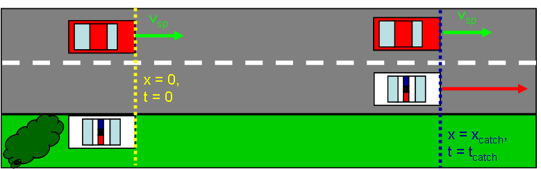
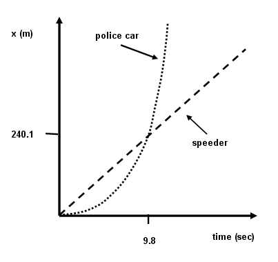
A speeder driving with a constant speed of 24.5 m/s approaches a (hidden) stationary police car on a long, straight road. The police officer detects the speeder using radar, and so the instant the speeder passes the police car, it begins accelerating after the speeder at a rate of 5.00 m/s2. How long will it take for the police car to catch up to the speeder from the instant its acceleration begins?
Solution
Systems:
There are two separate systems here. Both the police car and the speeder's car will be treated as point particles.
Interactions:
The police car experiences a constant acceleration as a result of the action of the pavement against its wheels.
Models:
The motion of the speeder's car will be modeled as One-Dimensional Motion with Constant Velocity. The motion of the police car will be modeled as One-Dimensional Motion with Constant Acceleration.
Approach:
Part B
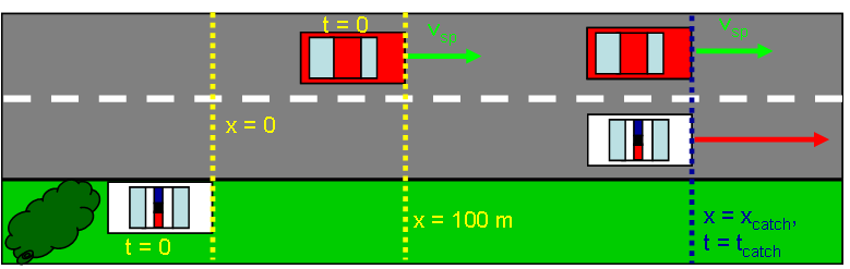
Again, a speeder driving with a constant speed of 24.5 m/s approaches a (hidden) stationary police car on a long, straight road. The police officer detects the speeder using radar, but this time the police officer begins accelerating at a rate of 5.00 m/s2 only after the speeder has progressed 100 m down the road (the speeder has a 100 m head start). How long will it take for the police car to catch up to the speeder from the instant its acceleration begins?
Solution
Systems, Interactions and Models: The same as for Part A.
Approach: