Return to Learning Curriculum
LS5: Engine Cooling Design
Lecture Zoom Recording
Original Author: Alexander Hodge '22, ahodge@mit.edu
- Note: This learning set looks at heat transfer in rocket nozzles, and how to design different engine cooling methods to keep the engine cool.
- Great Links
Introduction
Why Learn about Heat Transfer?
The general problem to solve is high temperatures in the combustion chamber, as these products of combustion are really hot (upwards of ~3000K, or 5000F!), so hot that it is above the melting temperature of virtually all metals. The job of the cooling designer is to keep engine metal below the material limits. This means that the cooling designer must understand how to effectively transfer the heat away from the combustion gas.
What is Heat Transfer?
‘Heat transfer’ is the transfer of heat from one place to another. Thermodynamic laws (i.e. the second law of thermodynamics) say that heat always flows in the direction opposite to the temperature gradient, meaning heat will flow from hot to cold temperatures. How much heat will flow depends on the type of heat transfer.
Heat Transfer Basics
Some Helpful Terminology:
Heat Transfer Rate: Q [W]
The rate of heat transfer looks at how much heat is getting moved or transferred across the mediums.
Heat flux: q [W/m2]
Also the same as Q/A. It is more commonly used when talking about heat transfer because it is independent of area, which is usually constant.
“Heat transferred”: Q*t [J]
This is the amount of heat that is transferred over some period of time. This isn’t used as often in hand calcs or derivations since it is time-dependent but good to know.
Temperature: T [K]
You know what temperature is. Just want to emphasize that in my unbiased opinion, Kelvin is the best unit to use for temperature. Ditch imperial units!
Types of Heat Transfer
Literature generally distinguishes between 3 types of heat transfer:
Conductive heat transfer
Convective heat transfer
Radiative heat transfer
Conductive Heat Transfer
Conductive heat transfer happens inside and through materials. The conduction equation is shown as:
This equation describes that the heat flux due to conduction depends on the conductivity of the material, and the gradient of temperature (not the change!) The gradient in simple terms is the slope of temperature/distance and is a vector operator in 3D. If we consider 1-dimensional heat transfer, we can write the conduction equation in some more friendly forms:

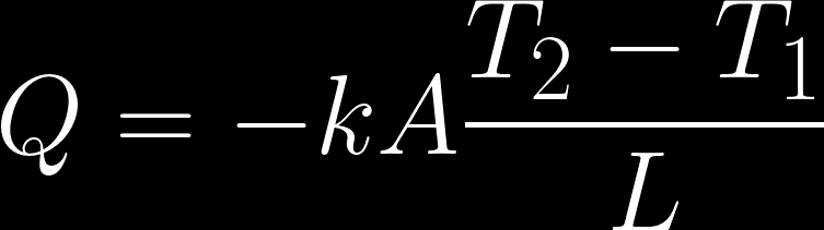
We can understand these equations better by looking at a simple example. In the example below we have a rod, connecting two reservoirs: the hot reservoir has temperature T2 and the cold reservoir has temperature T1.

We have a temperature gradient across the rod in the x-direction: 𝛿T/𝛿x = (T2-T1)/d and this means that heat will flow through the rod, from the hot side to the cold side. We can rewrite the equation for heat transfer as: q = -k*(T2-T1)/d
The proportionality constant between the amount of heat transfer and the temperature gradient is called the thermal conductivity, k.
A Quick Look at Unsteady Conduction (more complex)
Turns out, the full conduction equation is a lot more complex. In general, for the analysis in this unit, we are looking at simplified versions of the problem in order to make it possible for us to model the problem. In actuality, there are 3D and time-dependent effects that require much more complex equations and advanced algorithms to solve. Here is the full transient 3D conduction equation:

We get around having to use this equation by making 2 key assumptions:
Assume steady-state heat transfer (dQ/dt = 0)
Assume single-axis heat transfer
Turns out, it is easy to justify these assumptions while still making fairly accurate predictions on heat transfer in real-world applications. To learn more about how to justify these assumptions, or how to model more complex heat transfer, take a class like 2.51, 2.55, or 2.29.
Convective Heat Transfer
Convective heat transfer is the transfer of heat between a stationary and moving material. The easiest example to think about is a stationary plate with air flowing over it.
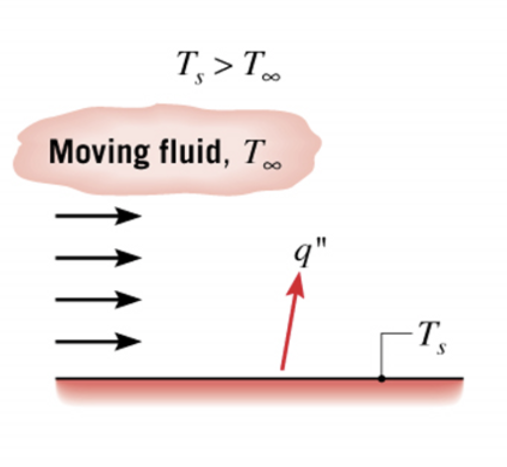
Imagine we have a cold fluid moving along a hot wall as shown above. Heat is being transferred from the wall to the fluid
The Fluid Boundary Layer
As the fluid is flowing along the wall, the fluid right at the surface of the wall will be stationary, while the fluid further away from the wall will be moving at velocity U. At the wall we have a ‘non-slip’ condition, meaning the particles cannot move there. This non-slip condition causes a thin layer along the wall with slow-moving fluid, namely a boundary layer.
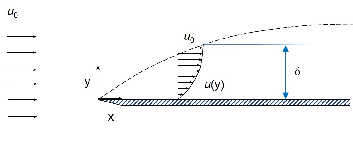
The above diagram shows the boundary layer thickness (𝛿), and the velocity profile as it decreases to 0 at the wall. Convective heat transfer happens through this thin layer of (almost) stagnant fluid.
The equation for convective heat transfer can be shown as:
(or)
We can see that this equation seems very similar to the equation for conductive heat transfer, namely a temperature difference times a coefficient, the heat transfer coefficient. Let’s now look at these terms in detail:
T2 would be the temperature at the wall surface
T1 would be the temperature of the fluid and the end of the boundary layer. This is a temperature in the fluid that is responsible for the heat transfer to the wall.
The heat transfer coefficient h. This coefficient depends on the type of flow over the plate.
Heat Transfer Coefficient
The heat transfer coefficient is very similar to the material conductivity, basically expressing how efficient heat is being transferred from the fluid to the wall.On a molecular level, heat transfer happens because molecules are moving around and they interact with the plate, giving off or receiving energy from the plate. You can imagine that the heat transfer from a very turbulent flow with lots of whirls would be different from the heat transfer from a very smooth flow.
To know the exact value of this heat transfer coefficient we, therefore, need to really understand the flow over the particular wall. Unfortunately, we still can’t predict with full certainty what the heat transfer coefficient will be. As a solution, a lot of people have conducted experiments and have come up with correlations for this heat transfer coefficient for very specific cases. When calculating heat transfer, you can look up a correlation that fits your case and use that.
As the heat transfer is very dependent on the type of flow, the correlations that are used to calculate the heat transfer coefficient involve properties of the flow, like Reynolds number, Prandtl number, and Nusselt number … These numbers are basically descriptions of the flow behavior. We’ll go over a few uses specific to rocket engine cooling a bit later, but you’ll learn more about these numbers in your fluids, thermo, and heat transfer classes.
Radiative Heat Transfer
Radiative heat transfer involves the electromagnetic emission of photons from objects. This is happening all the time, but when temperature differences are very low, radiation heat transfer is very low as well. The equation for radiation heat transfer illustrates this:
Because temperature is to the fourth power, and the Stefan-Boltzmann constant is so small (~5.7*10-8) only very large temperature differences will result in significant radiative heat transfer.
A good example of radiative heat transfer is the way the Sun transfers heat towards us on Earth. The sun is uber hot, and its glow is due to its radiation in the visible spectrum. Extremely hot metal that glows red illustrates the same phenomenon. Turns out, radiation happens in more than just the visible spectrum as well (ultraviolet, infrared, gamma rays, etc.). Although you can’t see it, it’s important to know that it is there, and model for it accordingly when necessary. This has huge impacts on the design of Earth-orbiting satellites!
Emissivity
The best way to affect radiative heat transfer is by changing the emissivity of the surface. A “black body” or “black body radiation” is an assumption used with radiation where we assume the emissivity ε = 1. We can get close to an emissivity of 1 by adding a dark layer on the outer surface. We can also get low emissivities by using shiny or polished metals, which will lower the radiation heat transfer (this is why aluminum foil is used to keep food hot/cold!)
Engine Cooling Methods
Heat Sink Cooling
When using a heat sink cooling scheme, the main thing being leveraged is the transfer of heat through physical material. In this setup, the heat from the combustion chamber and surrounding areas get absorbed into the chamber wall in order to reach a point of equilibrium with its resting temperature. In order to do so successfully, the area of high heat must be surrounded by a significant amount of bulk material so that the heat can transfer effectively while keeping the metal below its melting point.
Inherently, this is a very unstable problem due to the fact that tracking the exact transfer of heat through a material isn’t necessarily well defined. Because of this, heat sink cooling schemes require the engine to be constructed out of materials that have the following properties:
High Conductivity
High Density
High Heat Capacity
These properties combine in a value called the thermal diffusivity (𝛼): k/𝝆c [m^2/s]
The thermal diffusivity can be used in unsteady heat transfer calculations to see how the temperature evolves in time. This is extremely useful for modeling heat sink cooling methods, which often operate on lower time scales. This is because eventually, the entire object will reach thermal equilibrium, at which point you no longer have the heat transfer you need to keep the material from melting!
Although we have used this cooling method with the Helios engine, it is usually not implemented in industry unless the engine is rather small, has short firing times, and the temperature doesn’t need to be heavily regulated.
Radiative Cooling
Although slightly similar to the heat sink cooling scheme, a radiative cooling system focuses on radiating heat to the engine’s surroundings rather than to the material directly. Being the primary cooling method for cooling while in the vacuum of space, it relies on the nozzle being made out of a material with high emissivity. This allows the heat to be transferred out of the material and into its surroundings as soon as possible to cool down the entire system.
In order to optimize the performance of this type of cooling system, designs usually include very thin material to improve conduction, a convex body to improve heat transfer across the entire nozzle, and a highly emissive external coating.

In most real applications, this coating is simply coating the external walls of the engine with a very dark opaque material to facilitate expedited heat transfer to the surface that comes into contact with the vacuum of space.
However, given that the heat must still pass through the nozzle material, it’s very important to design a radiative engine with a high emissivity material in mind. That way, when combining the external coating with an already highly heat conductive material, you can maximize the heat transfer from the nozzle wall to the external surroundings. With this in mind, view the table below and ask yourself the following question: what material would be the best for a radiatively cooled nozzle? Use google to look up material conductivities! (Use your cursor to highlight the text after “Answer” to see the solution)

Answer: Copper with a Black Paint Coating
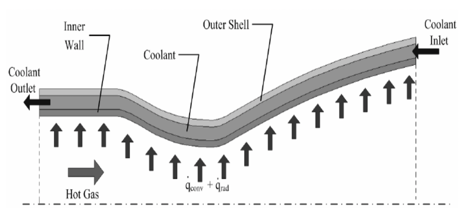
Regenerative Cooling
A regenerative engine cooling scheme is a system that passes the cryogenic propellant through the engine wall to cool the material before delivering it to the injector/combustion chamber.
It is called a regenerative cooling system because we use the fuel as coolant, before injecting it into the combustion chamber. In such a system, we are mainly concerned with conductive and convective heat transfer.
Convective heat transfer between the hot combustion gases and the nozzle wall.
Conductive heat transfer through the nozzle wall.
Convective heat transfer between the nozzle wall and the coolant.
This is illustrated in the figure below:
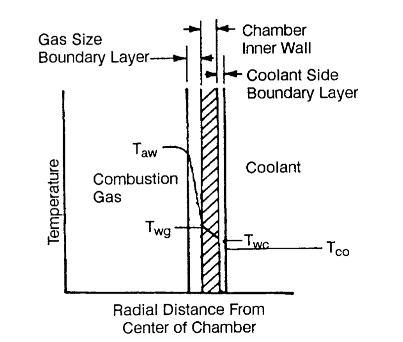
If we have a coolant temperature and a gas temperature, we can calculate how hot our wall will get by using the previously mentioned equations. The boundary condition is that the conductive heat flux from the gas to the wall will equal the conductive heat flux through the wall and also be equal to the heat flux from the wall to the coolant.
Actual designs of regenerative cooling systems usually involve a series of small channels that are lined circumferentially around the combustion chamber and nozzle.
Looking at a single channel, the coolant enters at some point along the engine profile, where it is pumped through at a high pressure and velocity. The coolant then exits the channel where it is eventually fed back into the injector, or sometimes dumped off as exhaust. There is a multitude in varying designs in regenerative cooling systems, which broadly involves:
Choice of channel entry/exit point
Number of channels
Location of cooling channels along the nozzle (sometimes only part of the nozzle/chamber is cooled)
Direction of coolant flow (exit plane -> injector plane, or vice versa)
So much more!
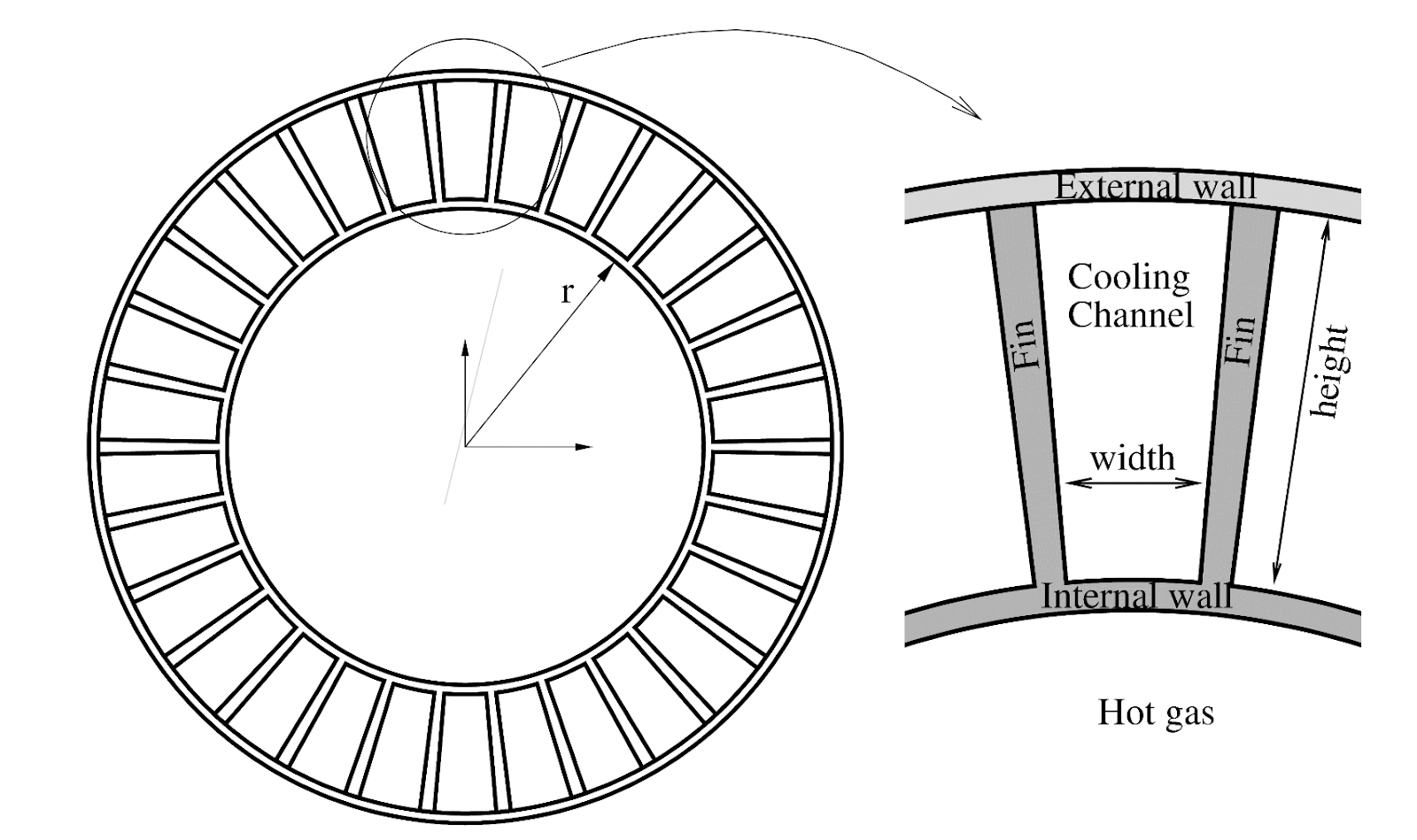
The geometry of the series of channels involves a few different geometric parameters as well:
Chamber wall (internal wall) thickness: We want to decrease this value to get better conduction, but are limited by the structural integrity and machinability of the material and structure.
Channel Rib (fin) thickness: We want this value to be small as well so that the fins can conduct heat from the chamber wall to the coolant.
Channel height & width: These parameters affect the cross-sectional area and aspect ratio of the channel (an aspect ratio of 1 is a square channel). To get better convective heat transfer, we want to have many small channels, as this will increase coolant velocity.
When designing regenerative cooling systems, the heat transfer coefficients are very important to keep in mind. In our case, we have a hot side and cool side HTC, and these values can be tweaked to adjust the temperature profile along the wall and boundary layers. Since the goal of engine cooling is to keep the material temperatures low, we will want our hot-side wall temperature to be as low as possible. This means that we will want to keep our hot side HTC small, and cool side HTC large. We won’t talk in-depth about heat transfer coefficients here, as the equations get quite intense, but understanding that we want hc / hg to be very large is a good first step in understanding the manipulation of these values to get a desired temperature.
Thermal Resistance Network
A relatively simple and common way to model networks of heat transfer is to use the circuit analogy. Here, we employ the circuit law equation and replace them with variables relevant to heat transfer:
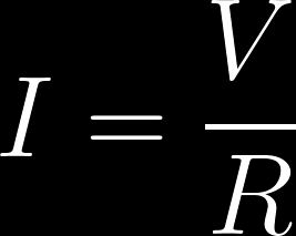

Current is analogous to heat transfer. Flow of electrons -> flow of heat
Voltage is analogous to temperature. Voltage drop -> temperature drop
Resistance is analogous to thermal resistance, and the expression changes depending on the type of heat transfer
For conduction and convection, we can easily derive the equations for thermal resistance:
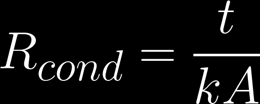

Now, using the circuit analogy, we can consider more complex heat transfer problems by considering different bodies and mediums to be resistors. Two pieces of material next to each other could be considered as two resistors in series, so we could find the equivalent resistance by adding the two thermal resistances (resistance add in series).
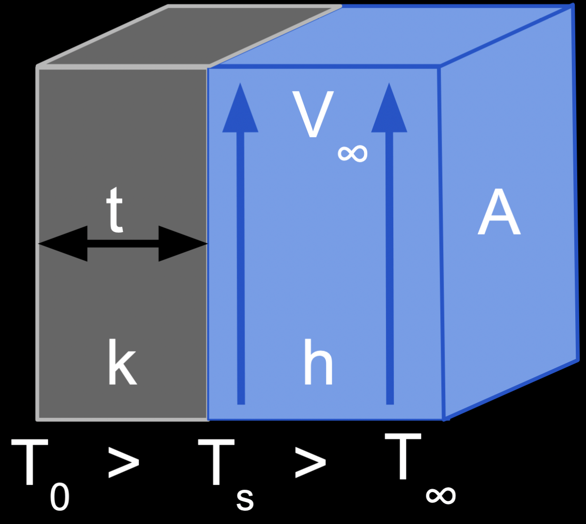
We can use thermal resistances to calculate the value of Ts , shown in the figure above. If we know T0, T∞, k, h, and A, we can find the thermal resistance of the grey material section (conduction), and the blue fluid section (convection). If we calculate the equivalent resistance, we can plug that into the heat flux equation to get heat flux, and then look at just the material section to back Ts, knowing the heat flux is constant.
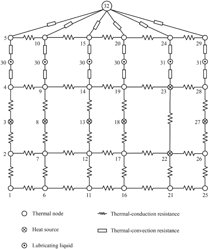
Thermal resistance networks have a huge use in industry, and they are also the fundamental basis for heat transfer modeling. Imagine a complex heat transfer problem (like the figure above) where you cut up the volume or area of interest into small cubes, define a thermal resistance in each direction, and then run a fancy algorithm that can look at each cell and/or node to find the temperature mapping everywhere!