The General Circulation of the Atmosphere
Introduction
The circulation of the atmosphere across the globe is chaotic; as a result, long-term weather prediction is theoretically impossible. However, large-scale structures in atmospheric circulation are stable over time and can be described by basic ideas about energy balance in the Earth system.
These constraints are explored in three other tank experiments described on this wiki: Balanced Motion, Fronts and Convection. Bringing these concepts together into a general circulation model explains the existence of some persistent features of the atmosphere, including the subtropical and polar jet streams, the trade winds, and the midlatitude bands in which rotating weather systems can be observed.
Theory
Balanced Motion
The Balanced Motion experiment develops three kinds of force balance: hydrostatic balance in the vertical, and geostrophic and cyclostrophic balance in the horizontal. It also introduces the Rossby number as a tool to determine whether geostrophic or cyclostrophic balance dominates in a given system.
Hydrostatic balance relates the pressure at a given surface to the weight of fluid above it.
| p = \rho g (H - z) |
Geostrophic balance is between the Coriolis force and the pressure gradient force, and dominates when centrifugal force is small.
| 2 \Omega v_\theta = g \frac{\partial h}{\partial r} |
Cyclostrophic balance is between centrifugal force and the pressure gradient force, and dominates when the Coriolis force is small.
| \frac{v_\theta^2}{r} = g \frac{\partial h}{\partial r} |
Whether geostrophic or cyclostrophic balance is a better approximation is determined by the Rossby number, which is simply the ratio of centrifugal to Coriolis forces in a system.
| R_O = \frac{|V_\theta|}{2 \Omega r} |
Tank Experiment
Two rotating tank experiments were set up. Tank rotation speed was the important parameter varied: one tank rotated at a speed of 1 rad s^{-1} and the other at 0.1 rad s^{-1}.
Slow Rotation Experiment
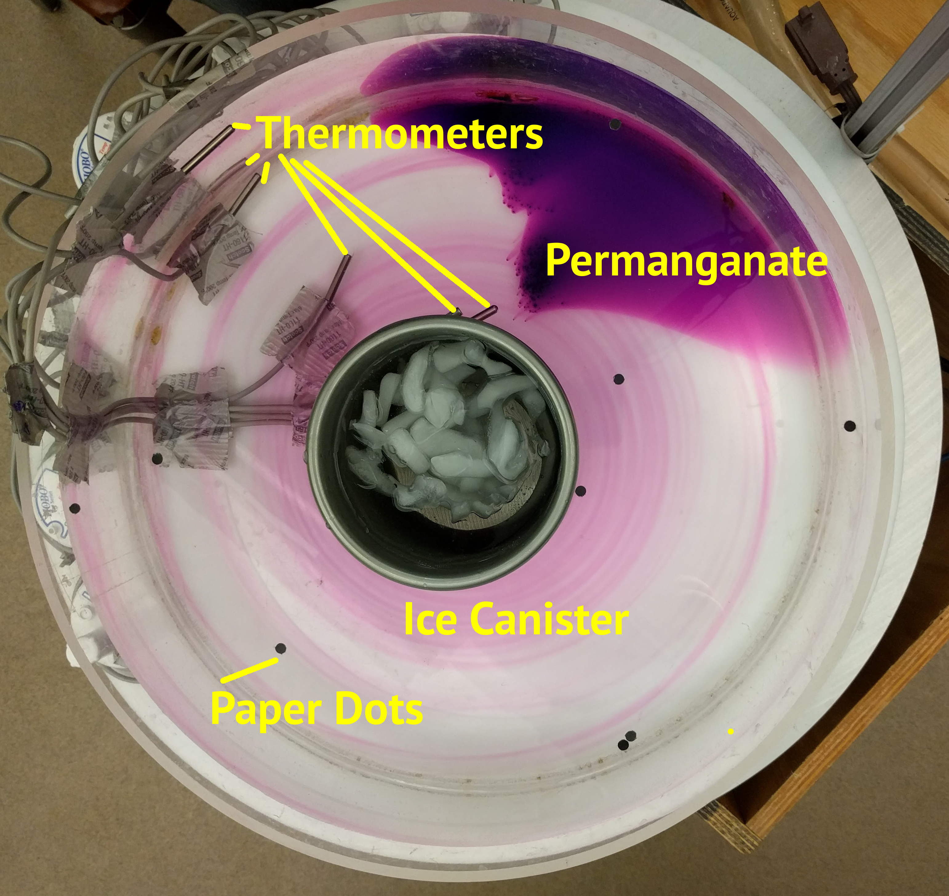
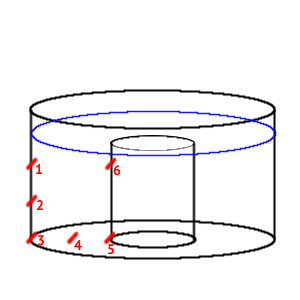
A metal canister of radius 12 cm was placed in the center of a tank of radius 22 cm. Six HOBO temperature sensors were taped to the tank in the arrangement shown in the figure below. The thermometer cables were taped along the bottom and edge of the tank to minimize interference with water flow. The tank was filled with still water to a height of 12.6 cm.
The rotating table was spun up to 0.1 rad s^{-1} and allowed to spin until a paper dot placed on the surface of the water appeared motionless to the overhead corotating camera, which was physically attached to the rotating table. The canister was filled with ice until full and then with water.
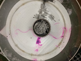
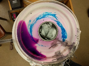
The surface speed of the water was measured by tracking black paper dots in the Particle Tracker application. The speed on the tank floor was measured by tracking the purple pigment trails from granules of potassium permanganate using timecoded screenshots in the Particle Tracker. Water speed shear between the top and bottom of the tank was measured with drops of blue food dye.
Fast Rotation Experiment
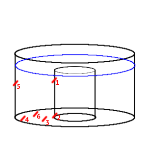
A metal canister of radius 18 cm was placed in the center of a tank of radius 31 cm. Again six HOBO temperature sensors were taped to the tank in the arrangement shown in the figure below. This arrangement differs from the first experiment: thermometers 1 through 5 were placed in a line radially from the tank center; thermometer 6 was placed between 3 and 4, on the bottom of the tank but 10 cm further in the clockwise direction. This arrangement was devised to capture thermal signatures of the eddies that were hypothesized to form. Thermometer 1 was placed at a height of 11 cm and thermometer 5 at a height of 9 cm. The tank was filled with still water to a height of 14 cm with water
The rotating table was spun up to 1 rad s^{-1} and allowed to spin until a paper dot placed on the surface of the water appeared motionless to the overhead corotating camera. In this setup, the speed of the corotating camera was synced electronically with the table rotation speed through a computer interface. The canister was filled with 521.6 g of ice and then with water.
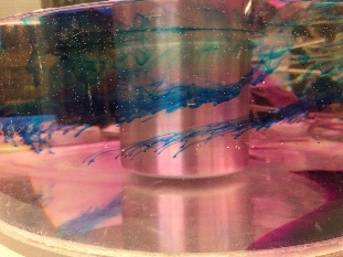
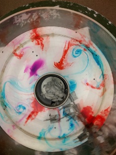
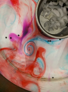
Surface speed, bottom speed and shear were measured as in the previous experiment: paper dots, permanganate granules and food dye, respectively. Two colors of food dye were used to illustrate eddy formation: blue dropped in the colder water near the canister and red in the warmer water near the outside edge.
Results
Slow Rotation Experiment
Fast Rotation Experiment
Bibliography