By: Beatrice Nash and Bethany Cates
1 Introduction
For our Dig Deeper Project, we wanted to build on our work from Project 3, where we examined the general flow dynamics created by the interaction of fluids of different air masses. In Project 3, we modeled the Hadley circulation as a two-layer system, but we didn't really think about how the boundary affected the fluid flow. Of course, fronts are really important for weather systems - most everyday weather phenomena occur at frontal boundaries. In this experiment, we investigated the frontal boundary more closely.
(TODO insert images of fronts in the wild)
2 Tank Procedure
3 Background theory: Thermal Wind and Margules relation
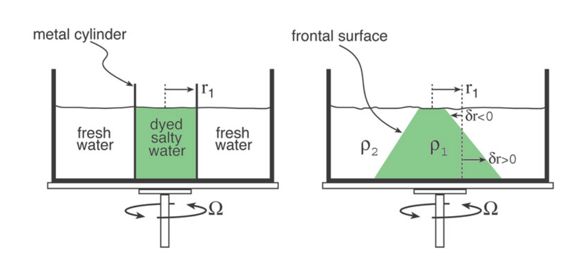
Figure 3.1: After the can is removed from the tank, the bottom of the dense fluid moves outwards, forming a cone. The less dense fluid converges towards the center of the tank, spiraling cyclonically in order to preserve angular momentum. The dense fluid spreads outwards, spiraling anti-cyclonically in order to preserve its angular momentum.-
4 Lab results
In order to collect data from our experiment, we tracked using video processing software buoyant particles at the surface of the fluid, as well as particles with density in between that of the two fluids which sat just above the frontal boundary. The shape of the front, although relatively stable, did vary slightly throughout the course of the experiment, as can be seen from the following images.
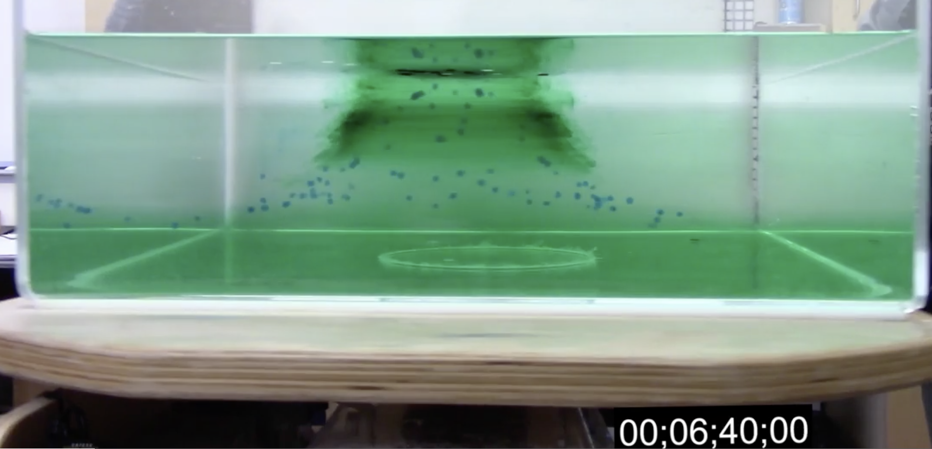
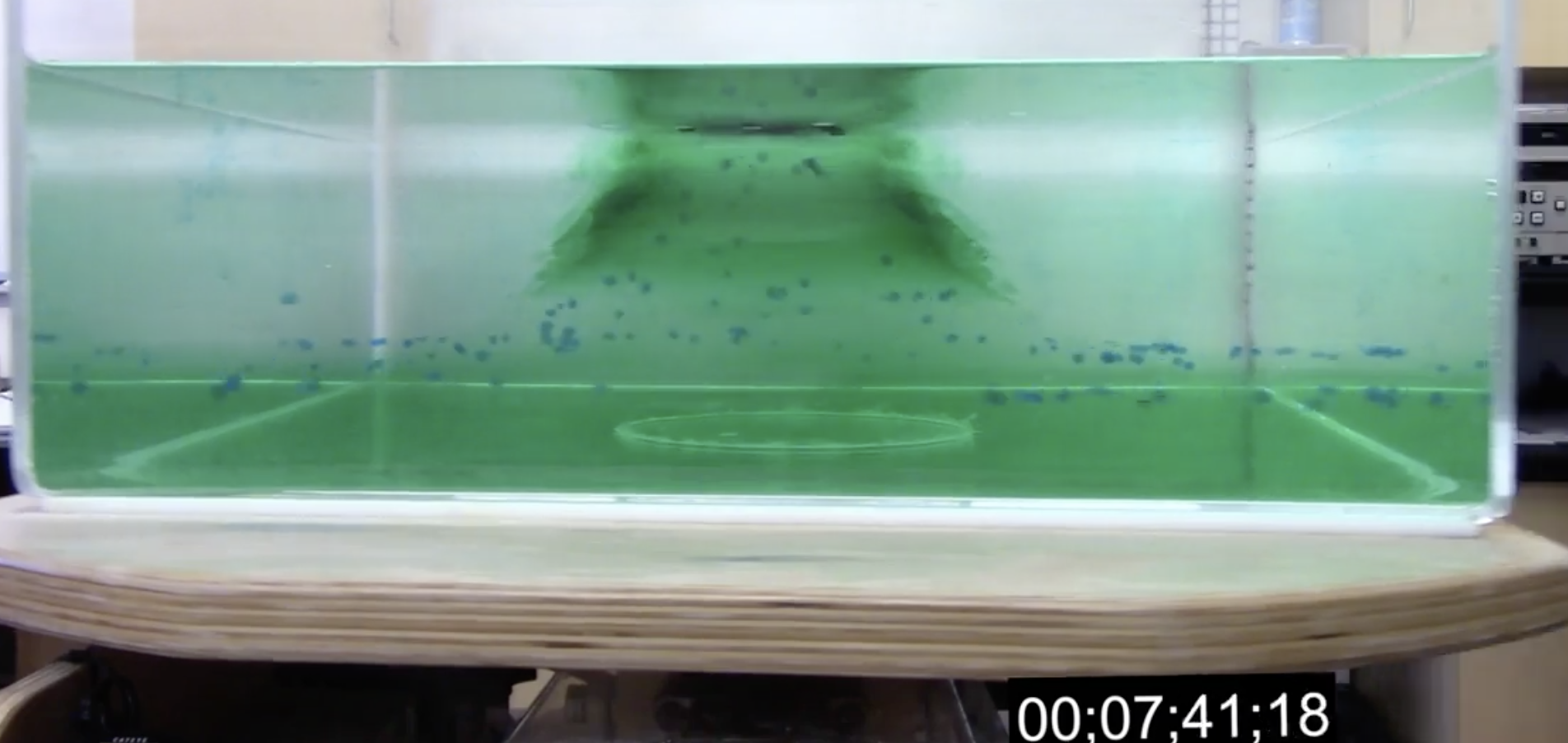
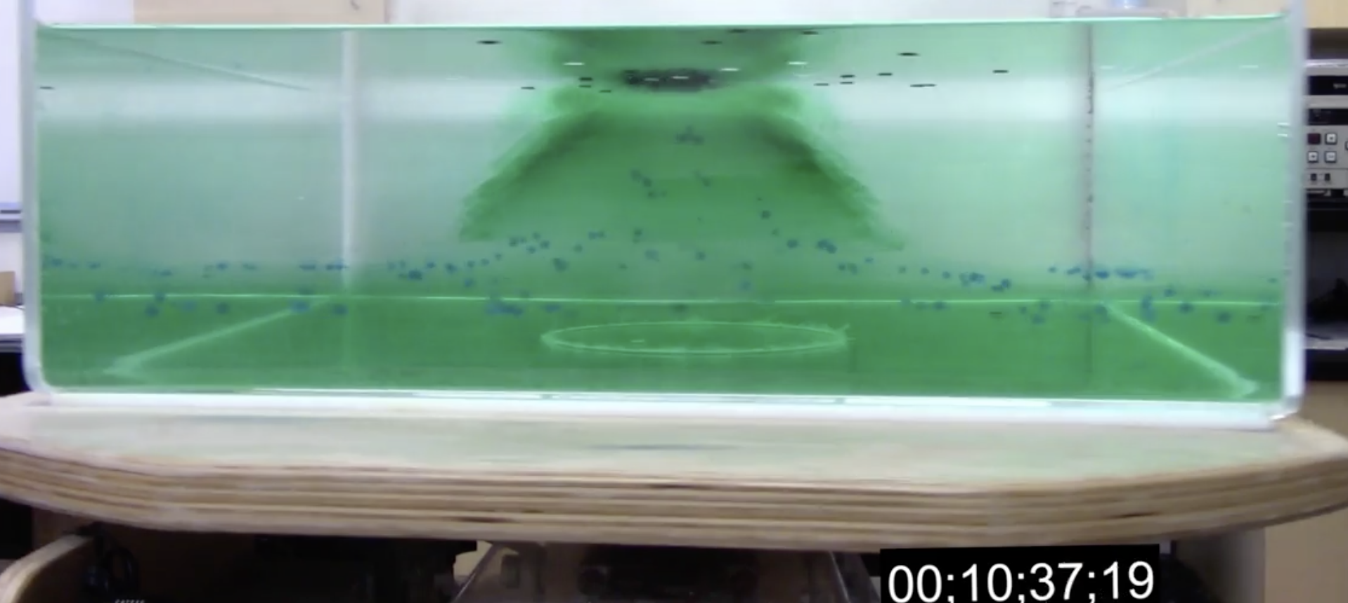
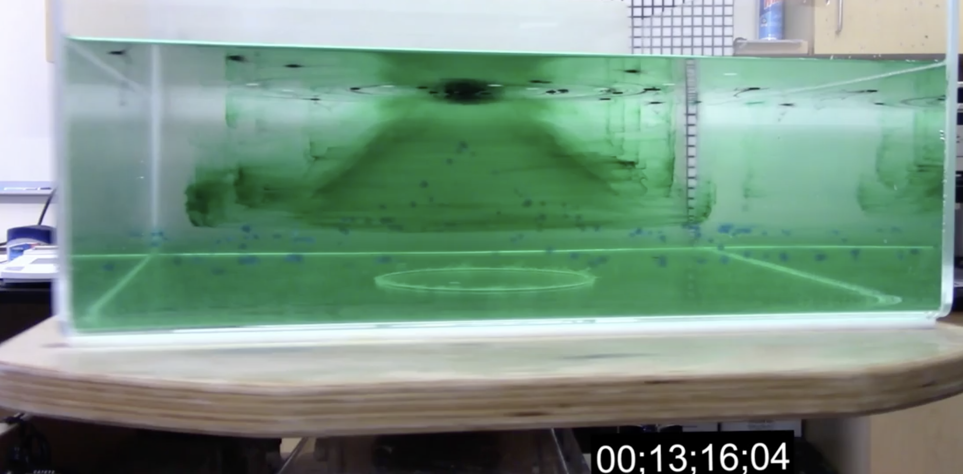
Figure 4.1: The progression of the front. The time stamp shown is relative to the time at which the can was removed.
Initially, the shape of the front resembles a Gaussian, with a wide sloping surface and flat top. As the experiment progresses, the frontal boundary gradually sinks relative to the free surface. Its sides flatten and the width of the center peak narrows.
Using equation x, we calculate the predicted radius of deformation to be around 20 centimeters, or half of the width of the tank. Since the boundary of the front extends all the way to the outside of the tank, about 3/4 of the distance to the bottom of the tank, the actual radius of deformation for this front is slightly larger than this prediction. Therefore, we see the slope of the front decrease towards the edge of the tank, as it has no more room to spread outwards.
Using the tracked particles, we now analyze the velocity of the fluid both on the surface and at the frontal boundary starting around 11 minutes after the removal of the can. As can be seen from the above images, the fluid appears sufficiently stable at this point in the experiment to assume hydrostatic balance. At this time, we track particles at the surface, resulting in the following set of tracks:
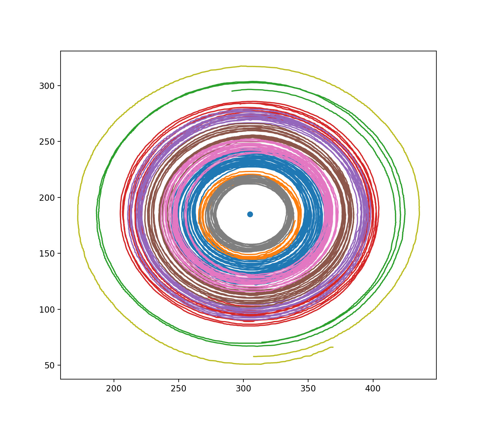 .
.
Figure 4.2: Trajectory of particles at the surface of the fluid tracked ≈11 minutes into the experiment, for ≈1 minute each. The axes are labeled in pixels, and the dot at the center indicates the center of the front. Each of the different colors corresponds to an individual tracked particle. The particles have small but noticeable radial displacement towards the center of the front.
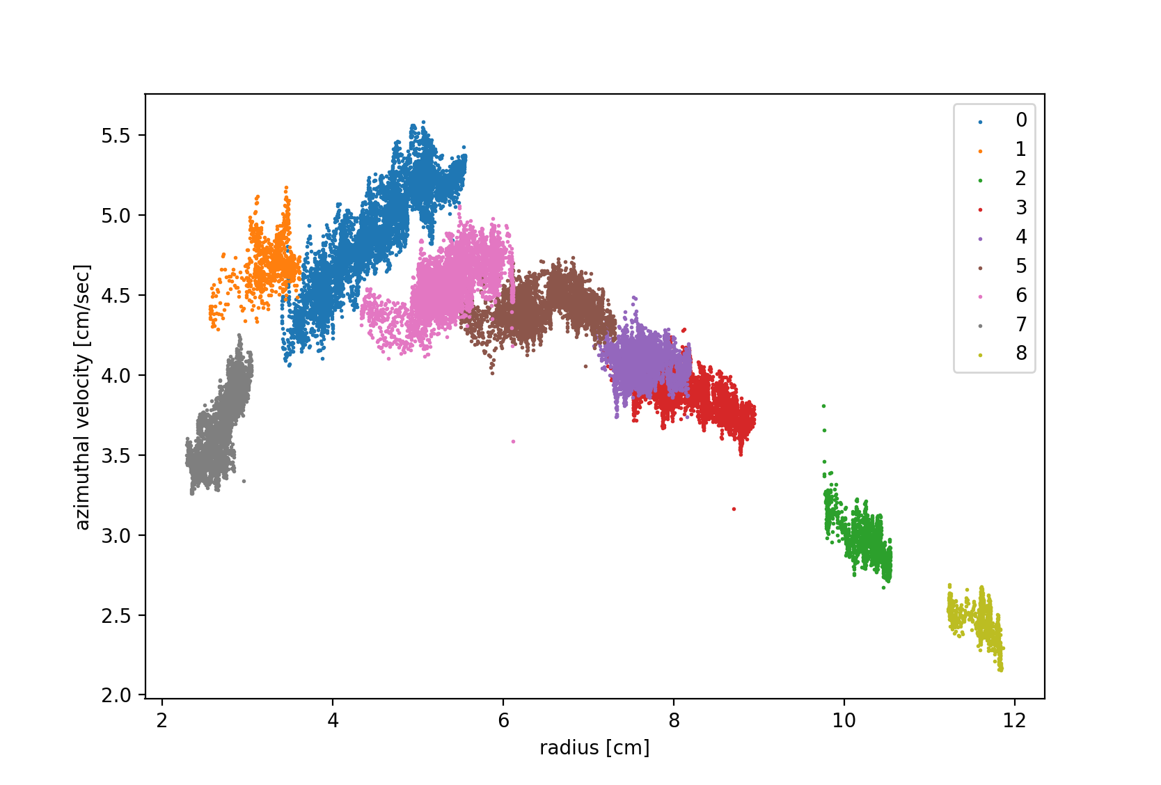
Figure 4.3: azimuthal velocity as a function of radius for the tracks shown in the Figure 4.2.
From the two above plots, one can see that the fluid does behave cyclonically at the surface, as we expected. At large radii, where the frontal boundary has a very small slope, the azimuthal velocity is small, as would be expected from the Margules relation. Notice that the maximum radius of the tracks is less than 12cm, whereas the edge of the tank is ≈20cm from the center of the front. At larger radii, the azimuthal velocity is nearly zero as the frontal slope is so small.
As the radius decreases, the slope increases and so does the azimuthal velocity of the fluid, reaching its peak at around 5cm. This radius approximately corresponds to the location of the edge of the can before it was removed. We would expect the pressure gradient at this radius to be largest, which implies fluid at this radius should also have the largest velocity (see equation y). At small radii, the azimuthal velocity decreases again as the frontal boundary flattens and the pressure gradient decreases.
We also track the particles which sit just above the frontal surface. These are the blue spheres seen in Figure 4.1.
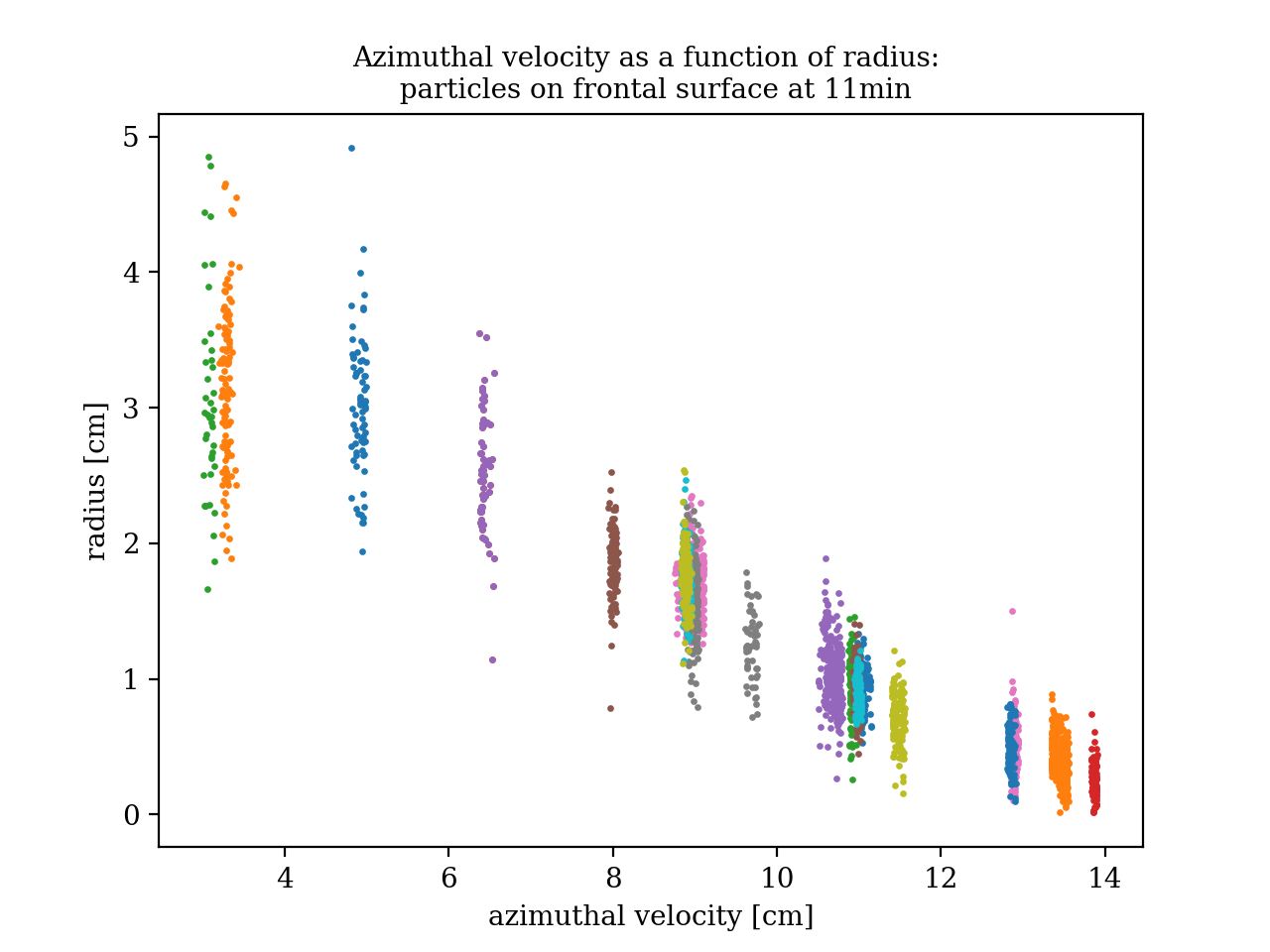
Figure 4.4: azimuthal velocity as a function of radius for particles tracked at the surface of the front.
These particles are more difficult to track, hence the tracks are shorter, and the concentration of dye and particles at the center of the front makes it impossible to track the particles for very small radii accurately. Still, it is clear from this plot that the azimuthal velocity of the fluid at the frontal surface has the same overall radial dependence as that of the fluid at the free surface for large radii. However, we see only a small peak at 5cm, unlike the very defined peak at that radius for the velocity of the fluid at the surface.
As expected, for the same radius, these particles have smaller azimuthal velocity than those at the surface. Upon removal of the can, the fluid at the surface is displaced towards the center more than the fluid at lower depths, therefore in order to preserve angular momentum the fluid at the surface must acquire greater azimuthal velocity.
Using the Margules relation and the data collected for the velocity of particles at the boundary of the front to solve for the frontal slope, we "backed out" what the boundary of the front would look like according to the theory.
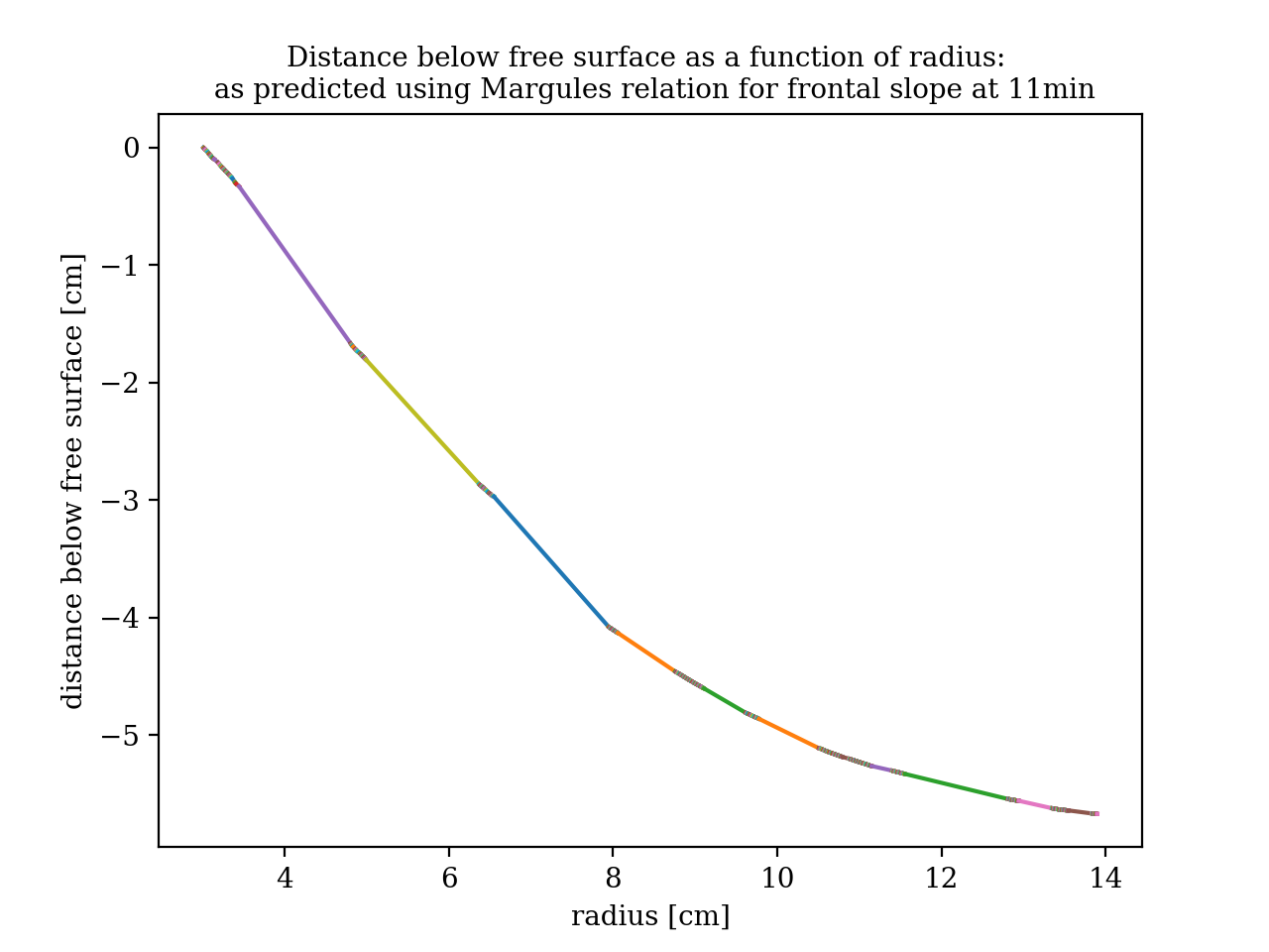
Figure 4.5: Predicted frontal boundary using the Margules relation at the velocity of particles tracked at the boundary. The particle with smallest radius was assumed to be near enough to the highest point of the frontal boundary. The largest radius of the tracked particles is about halfway between the center of the front and the edge of the tank.
Accurately comparing the images taken (Figure 4.1) to the plot above would be difficult due to issues of distortion. However, just looking at the 3rd image in Figure 4.1, the closest in time to when the particles were tracked, one can see that the overall shape of the front aligns well with the prediction. Therefore, we conclude that the Margules relation provides a good estimate for the shape of a front, given that the assumption of geostrophic flow holds.