The heart of the software is contained in the Extraction step, where essentially all of the heavy lifting occurs. It is a slow process, taking roughly 15 minutes per science frame on a fairly modern MacBook pro. During extraction, the following steps are performed:
- A 2D wavelength map is determined by matching each order to a template spectrum of the OH sky lines and/or ThAr arc lamp spectra. This produces an output file containing the log of the wavelength for each pixel on the array (and in an order). The wavelengths are corrected for heliocentric velocity shifts, and are in vacuum units by default (since the instrument is in vacuum).
- The software calculates tilt of the slit in each order for accurate sky subtraction.
- A first pass 2D sky subtraction is performed for the purposes of object finding.
- Each order is collapsed in the wavelength direction to locate the object trace. The trace is then fit over the full order.
- An iterative procedure is used to perform a simultaneous fit of both the object profile and background sky residuals.
- An optimally-weighted extraction is performed using the profile determined in (5).
- Spectra are stored on an order-by-order basis in units of counts vs. wavelength.
For high signal-to-noise ratio data, a non-parametric b-spline is fit to the object profile; at lower SNR a Gaussian model is used.
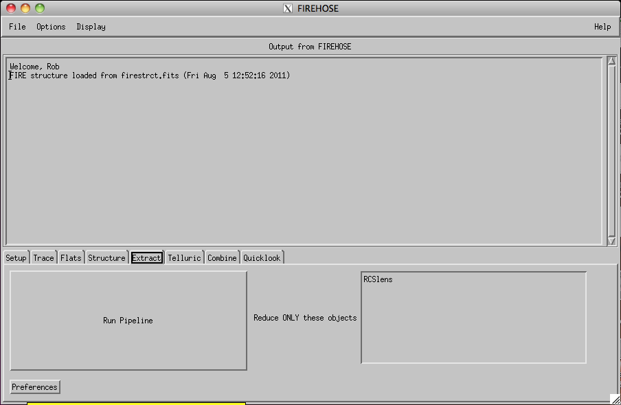
This process was fully automated in early versions of the pipeline but we have begun adding the ability to set user preferences for extraction. To edit the preferences, click the corresponding button on the lower left hand corner of the "Extract" tab:
This will bring up a separate preferences panel that looks like the following:
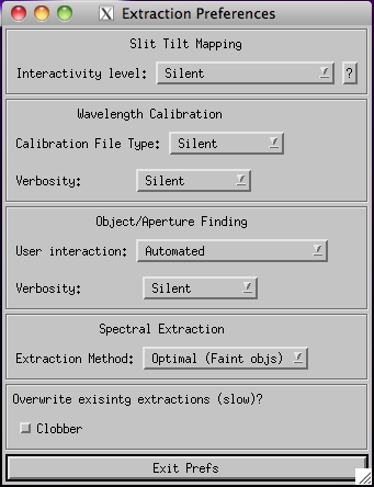
Ongoing development for the pipeline is currently focused on increasing the range of options available to the user, but at present a few have been implemented:
- Slit tilt mapping: Fit of the slit tilts is a critical part of the sky subtraction and wavelength calibration process. Usually this happens in the background but it is sometimes useful to see the results, particularly if an error has occurred downstream in sky subtraction. Setting this tab from "Silent" to "Inspect Results" allows you to see which lines were used to define the slit tilt and how the fit performed. This mode is very slow since it displays rectified arc images for each of the 20 orders one by one for each exposure. In normal operation it should not be used, only to diagnose problems, or to familiarize yourself with the pipeline on first use. Debug mode includes additional stops in the code and is generally not useful for non-experts.
- Wavelength Calibration file type: The default in FIREHOSE is to use the OH sky lines for slit-tilt mapping and wavelength calibration for exposures longer than 300 seconds. For those less than 300 sec, ThAr lamp exposures are used. Using this tab the user can force ThAr to be used for all exposures. In principle one could force OH for short exposures but in our expedience this has not worked well.
- Interactive Wavelength Fits: If you have lots of time on your hands, you can inspect the arc line fits for each order and each exposure interactively. Turning this on will pop up a GUI for each order's fit showing the automatic line IDs, and allowing you to add or reject points and adjust the fit by hand. Plan on spending an hour or more per exposure if you use this mode, but it does give you total access if you are a control freak. The GUI is much like iraf's reidentify. It is based on the x_identify.pro procedure distributed with xidl.
- Object/Aperture Finding: The FIREHOSE automated object finder works well for point sources with continuum detection in many/most orders. However if your exposure shows only emission lines, or has no continuum (but you know where it should fall on the slit), or if you want to force a particular aperture, then there are options to set the trace location and apertures by hand.
- User/interactive aperture definition: In the case where many orders have no flux but one or a few emission lines are visible, it is possible to define the aperture around these emission lines. There is a separate GUI associated with this operation. See this link for a page describing how to perform this operation.
- Reference Star tracing: This mode is useful when there is no flux visible from the science object, but you expect the science target to fall at the same slit position as a reference object (e.g. a blind offset pointing star, or a telluric standard star). It is available in beta mode only and the mechanism for associating reference star exposures with science frames is somewhat clunky. Nevertheless by popular demand we include information on how to run it at this link. Note that it is now possible to use this in conjunction with post-processing routines to make a rectified and flux-calibrated 2D spectrum that is appropriate for running extraction with your own routines.
- Extraction Options: The default mode is to extract optimally (a la Horne) using either a non-parametric weighting function fit to high-SNR data, or a Gaussian fit in the low-SNR regime. The user can change this option to run in straight boxcar mode as well (i.e. simple sum of flux within the defined aperture). Users observing bright objects, where saturation or high counts are an issue, will want to extract in boxcar mode. Users extracting faint objects will find better performance in optimal mode. Note that in optimal mode the sky subtraction performs better because FIREHOSE performs an iteractive local correction to the sky and object model to minimize sky residuals after the standard Kelson-style 2D sky subtraction. Boxcar does not perform this second iteration, but it does run much faster (10-15 seconds, as opposed to 10 minutes).
- Clobber toggle: By default the pipeline does not overwrite working and ancillary files during the reduction process, in order to save time. With this flag turned on, the full reduction is overwritten. This ensures a clean run but is slower. In future releases we plan to separate out the clobber functions for arcs, extraction, etc independently.
During extraction, you will see plots of the object profile appear to indicate data quality. The plots show a cross section of the object profile with errors, and the resultant fit. As the iterative model fit and local sky subtraction improve, you should see the residuals in this plot diminish, through each iteration on a given order.
Because this process is slow, it can take a day or more to reduce a full run or data. In many cases you are interested in a particular object. You can choose a subset of the full target list to extract to speed the process. To do this, simply highlight the names of the targets you want to extract given the list at right of the panel. If you have already reduced some of your frames, firehose will not re-reduce them unless the "Clobber" button is pressed.